Siddarth Ijju

Advanced Generative AI (Vision Series): VQ-VAE

Introduction

In my previous series, I covered the fundamentals of generative A.I. for vision - the VAE, the GAN, and the DDPM (if you haven’t seen those articles, you can find them on my blog). In this new series, I’ll explore more advanced versions and additions to the above algorithms, building up to the modern state of the art.

To start, this article explores the Vector Quantized Variational Auto Encoder, or the VQ-VAE. The VQ-VAE is a fundamental part of algorithms such as Stable Diffusion, so an understanding of the implementation and theory behind it is critical for modern image generation algorithms. Let’s dive in!

Vector Quantized Variational Autoencoders

Originally proposed in 2017, the vector quantized variational autoencoder (VQ-VAE) builds on top of the fundamental backbone of the VAE. If you’d like a review of the concepts behind the VAE, you can check out my earlier article here - for this article I’ll only provide a quick review before going through the theory.

The VQ-VAE addresses some fundamental problems with the VAE. First, the VQ-VAE uses a discrete latent space, which is more suitable for some applications such as language and vision than the continuous latent space used by the VAE. Second, the VQ-VAE simplifies the latent space, which helps reduce variance in the outputs and improve posterior collapse, which is a problem that often occurs with VAEs where the generated images look very similar to each other. Let’s analyze how the VQ-VAE accomplishes these objectives.

Setup

At its core, the VQ-VAE is very similar to the VAE. Both algorithms utilize an encoder network that takes as input some $x$ and outputs $z_e(x)$ , as well as a decoder network that performs the reverse procedure and outputs $\bar{x}$ from $z_e(x)$ .

In the VAE, we actually had our encoder output parameters $\mu$ and $\sigma$ to describe a multivariate normal distribution representing our latent space. As you can imagine, this is a very complicated latent space to use for many applications. The core idea behind the VQ-VAE is to replace the normal distribution representation of the latent space with a categorical distribution. Let’s see how this works.

Vector Quantization

We’ll use the concept of vector quantization to implement the idea above. Let’s first define a latent embedding space of vectors $e \in \mathbb{R}^{K \times D}$ , where $K$ represents the number of embedding vectors and $D$ represents the dimensionality of each latent vector. Our goal is to use vectors $e$ from this embedding space as representations of the latent instead of the raw outputs from the encoder.

Let’s assume that our encoder network outputs a vector of latents $z_e(x)$ . To quantize this output, all we need to do is select the closest vector from the embedding space, which we can do using metrics like the Euclidean norm or cosine distance. Then, instead of the original encoder output $z_e(x)$ , we’ll use this quantized vector, which we’ll label $z_q(x)$ as the input to the decoder. As a result, the posterior distribution can now be represented as a categorical distribution where
$q(z = k | x) = \begin{cases} 1 & k = \argmin_j{\lVert z_e(x) - e_j\rVert_2}\\ 0 & \text{otherwise}\\ \end{cases}$
We’ll choose embedding vectors via an algorithm inspired by $k$ -means clustering - we’ll assign each embedding vector to the center of the cluster of vectors that are assigned to it.

One problem the observant reader might realize is that using a latent space consisting of only $K$ different vectors will result in an algorithm only capable of producing $K$ distinct results. In practice, we fix this issue by using a field of latents instead of one singular latent. For example, if we use a field of 32 x 32 latents, each of which can take on $K$ different values, we would be able to represent $K^{1024}$ different outputs, which is more than enough to ensure sufficient sample diversity.

Another problem with the current approach above is that there isn’t an easy to define gradient for the argmin operation that we use to select the embedding vectors. Without gradients passing through to the encoder, we’d be unable to learn anything meaningful.

To resolve this, the authors utilize an approach known as straight-through estimation, which is basically a fancy way of saying “copy the gradients from one place to another”. There’s a lot of theory behind why this approach is good enough that I won’t go into now, but it’s sufficient for our purposes. In our case, we’ll just copy the gradients from the decoder inputs to the encoder outputs and use those to backpropagate for the encoder network.

Loss

With the vector quantization aspect of the VQ-VAE framework out of the way, we can now discuss the objective we’ll use to train this model.

First, let’s recall the objective from the vanilla VAE. We would like to minimize the Kullback-Leibler divergence between the estimated posterior distribution $q(z | x)$ and the true posterior distribution $p(z | x)$ . I’ll skip the detailed derivation (if you’d like to read through it, you can check out my VAE article), but this objective simplifies to maximizing the log probability of the data $\log p(x)$ , which has a lower bound known as the ELBO:

$\mathbb{E}_q \left[ \log \frac{p(x, z)}{q(z | x)}\right]$
which can also be written as
$-D_{KL}(q(z|x) \parallel p(z)) + \mathbb{E}_q[\log p(x | z)]$

The setup of the VQ-VAE allows us to do something quite nice here since we know that $q(z | x)$ is actually a deterministic categorical distribution $q(z = k | x)$ .

First, we can rewrite the KL divergence term from above as $\mathbb{E}_q[\log \frac{p(z)}{q(z | x)}]$ . We know that there is exactly one value of $z$ that $q(z | x)$ can take on for each $x$ , and that $q(z = k | x) = 1$ only occurs when $k = \argmin_j \lVert z_e(x) - e_j \rVert_2$ , and is $0$ otherwise. Furthermore, if we assume a uniform prior over $z$ during the training of the encoder and decoder, where each $z$ has a $\frac{1}{K}$ probability of appearing, we can then simplify $\mathbb{E}_q\left[\log \frac{p(z)}{q(z = k | x)}\right] = -\log K$
This implies that we can actually ignore the KL divergence term in our loss objective for the encoder and decoder, and simply focus on maximizing $\log p(x | z)$ . I won’t go into the derivation in detail here since I’ve covered it in earlier posts, but if we assume the true distribution $p(x | z)$ follows a Gaussian distribution, we can maximize this term by minimizing the mean-squared error between the reconstruction and the input.

Second, we require a term to ensure that the embedding vectors are good representatives of the latent space. Recall from earlier that the core idea behind vector quantization is the move the vectors in the embedding space to the clusters in the latent space that they represent the most. In mathematical terms, this is simply minimizing the average distance between each embedding vector and the vectors that we map to that vector to, which we can write as $\lVert z_e(x) - e \rVert^2_2$ .

However, we don’t want to update the encoder network with this term - we just want to update the vector quantizer. To implement this nuance, we’ll use an idea known as the stop-gradient function ( $sg(x)$ ), which is essentially a function that zeros out the gradients for that particular input. If we use the stop-gradient on the encoder output, this term of the objective then becomes
$\lVert sg(z_e(x)) - e \rVert^2_2$

Finally, the authors utilize an additional term in the loss function to prevent the encoder outputs from exploding. Since the encoder outputs aren’t directly used in the decoder, and since we’re only checking what vectors are closest to the encoder outputs in the embedding space, it’s possible for the volume of these vectors to increase unchecked. To prevent this from occuring, the authors utilize an additional term to ensure the encoder outputs are close to the embedding vectors, which is a mirror image of the term above.
$\lVert z_e(x)- sg(e) \rVert^2_2$
Here, we use the stop gradient on the embedding vector since we’d like to have the gradient flow through and improve the encoder. We also usually include a scaling constant $\beta$ to ensure that this term is prioritized properly compared to the other terms.

With the above three terms, we can now construct a complete objective.

$L = \log p(x | z) + \lVert sg(z_e(x)) - e \rVert ^2_2 + \beta \lVert z_e(x)- sg(e) \rVert^2_2$

where the decoder optimizes the first term, the encoder optimizes the first and third term, and the vector quantizer optimizes the second term.

Prior

We’re done with the main work, but there’s still a big question - how do we actually use this setup to generate new images? In the original VAE, we sampled from the multivariate normal distribution that the encoder outputted and then used that sample as input for the decoder. However, in the VQ-VAE, we no longer have an easy way to sample from the latent space. Furthermore, our assumption of a uniform prior over the latent space likely won’t hold up during generation.

The authors of the paper propose using a separate autoregressive model to learn the distribution of the latent space and generate valid latent samples. I won’t cover the full details here but the authors suggest using a PixelCNN (subsection in paper) to generate the latent maps for 2D inputs and outputs. PixelCNNs are very powerful models in the computer vision domain, so they’re good to know about but they require their own article to fully do them justice.

Implementation

We’ve now covered all aspects of the theory behind the VQ-VAE that we need to implement the model. Let’s dive right into implementing this structure in PyTorch.

Encoder and Decoder

First, we’ll implement the Encoder and Decoder modules. These modules follow a similar pattern to the original VAE, so for the sake of brevity I’ll simply put the code used to initialize the encoder and decoder.

Here, we initialize the encoder network as an instance variable of our VectorQuantizedVariationalAutoEncoder module.

	
self.encoder = nn.Sequential(
    nn.Conv2d(input_dim, dim, 4, 2, 1),
    nn.BatchNorm2d(dim),
    nn.ReLU(True),
    nn.Conv2d(dim, dim, 4, 2, 1),
    ResBlock(dim),
    ResBlock(dim),
)

The decoder follows a very similar structure, but in reverse.

	
self.decoder = nn.Sequential(
    ResBlock(dim),
    ResBlock(dim),
    nn.ReLU(True),
    nn.ConvTranspose2d(dim, dim, 4, 2, 1),
    nn.BatchNorm2d(dim),
    nn.ReLU(True),
    nn.ConvTranspose2d(dim, input_dim, 4, 2, 1),
    nn.Sigmoid()
)

One notable addition is the use of residual blocks in the encoder and decoder structure, which helps with the propagation of high-level features through the network. I’ve included the code for the ResBlock below.


class ResBlock(nn.Module):
    def __init__(self, dim):
        super().__init__()
        self.block = nn.Sequential(
            nn.ReLU(True),
            nn.Conv2d(dim, dim, 3, 1, 1),
            nn.BatchNorm2d(dim),
            nn.ReLU(True),
            nn.Conv2d(dim, dim, 1),
            nn.BatchNorm2d(dim)
        )

    def forward(self, x):
        return x + self.block(x)

Vector Quantizer

Next, we’ll tackle the vector quantizer module. We’ll set this module up as a container for embeddings defined by the input parameters $K$ and $D$ . We’ll also implement separate methods to embed inputs of a particular shape, in addition to the standard .forward method so that we can update our embeddings with PyTorch’s autograd functionalities. Here’s the full code for the module:

	
class VectorQuantizer(nn.Module):

    def __init__(self, K=512, D=64):
        super(VectorQuantizer, self).__init__()
        self.K = K
        self.D = D
        self.embeddings = nn.Embedding(K, D)
        self.embeddings.weight.data.uniform_(-1./K, 1./K)

    def embed(self, indices, shape):
        quantized = torch.index_select(self.embeddings.weight, 0, indices).view(shape)
        quantized = quantized.permute(0, 3, 1, 2).contiguous()
        return quantized

    def forward(self, x):
        x = x.permute(0, 2, 3, 1).contiguous()
        flattened = x.view(-1, self.D)

        distances = torch.cdist(flattened,self.embeddings.weight)
        indices = torch.argmin(distances,dim=1) 
        indices = indices.reshape(x.shape[:-1])

        return indices

One key item to notice here is that the forward method doesn’t return the actual embeddings. Instead, the forward method returns the indices of the corresponding embedding vectors. This will be useful for our implementation of the overall encode method, and in our training for the prior model.

PixelCNN

The PixelCNN module will be used as our implementation of the learned prior for the overall VQ-VAE. Since most of the code for this module isn’t relevant for the main VQ-VAE, I’ll skip past it for this article but if you’re curious, you can check out the implementation in my public repository.

One relevant block to note is the sample method of the PixelCNN, which will be used to generate priors of shape (32for input into our decoder.

	
@torch.inference_mode
def sample(self, n, shape=(32, 32)):
    param = next(self.parameters())
    x = torch.zeros(
        (n, *shape),
        dtype=torch.int64, device=param.device
    )

    print("### Generating prior ###")
    with tqdm(total=shape[0] * shape[1], position=tqdm._get_free_pos()) as pbar:
        for i in range(shape[0]):
            for j in range(shape[1]):
                logits = self.forward(x)
                probs = F.softmax(logits[:, :, i, j], -1)
                x.data[:, i, j].copy_(
                    probs.multinomial(1).squeeze().data
                )
                pbar.update(1)
    return x

Bringing it all together

Now that we have each sub module implemented, we can put them together to write our encode, decode, and forward methods for the overall VectorQuantizedVariationalAutoEncoder module.

The encode and decode methods are relatively straightforward. The encoder outputs the discrete latents as indices of embedding vectors, and the decoder embeds and then generates outputs from those latents.

         
def encode(self, x):
    z_e_x = self.encoder(x)
    latents = self.vq(z_e_x)
    return latents

def decode(self, latents):
    z_q_x = self.vq.embed(latents, (-1, 32, 32, 256))
    x_tilde = self.decoder(z_q_x)
    return x_tilde

The forward method is a bit more nuanced. In the vanilla VAE, we could essentially just call the encoder and decoder in order, but recall that we must implement straight-through gradient estimation to copy gradients from the decoder to the encoder for the backward pass of the VQ-VAE. We’ll implement this using PyTorch’s .detach functionality as follows.

    
def forward(self, x):
    z_e = self.encoder(x)
    latents = self.vq(z_e).view(-1)
    z_q = self.vq.embed(latents, (-1, 32, 32, 256))

    # straight through gradient
    st_z_q = z_e + (z_q - z_e).detach()

    x_hat = self.decoder(st_z_q)
    return x_hat, z_e, z_q

Generating Art

Now that we have every module written, we can put together a quick training loop and dataset to generate some cool new images!

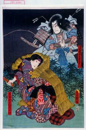
As always, all the experiments below use images from the Japanese Woodblock Print database to better emulate the challenge of handling real datasets in the wild.

ukiyo-e sample

Let’s try and generate images like the one above!

I’ll skip the steps of defining the dataset and dataloader since they’re usually pretty simple and instead focus on the training loop for the VQ-VAE. If you’d like to see that code, you can check out the full repo here .

Let’s define our actual training loop. In this case, we’ll have two separate loops - one for the prior model and one for the main VQ-VAE itself. Here’s the loop for the VQ-VAE alone:

    
vq_vae = VectorQuantizedVariationalAutoEncoder()
vq_vae.to(device)
optimizer = optim.Adam(vq_vae.parameters(), lr=lr, betas=(0.5, 0.999))

for epoch in tqdm(range(n)):
    for i, batch in enumerate(self.dataloader, 0):
        batch, _ = batch
        batch = batch.to(device)

        vq_vae.zero_grad()

        batch_hat, z_e, z_q = vq_vae(batch)

        reproduction_loss = F.mse_loss(batch_hat, batch)
        dictionary_loss = F.mse_loss(z_e.detach(), z_q)
        commitment_loss = F.mse_loss(z_q.detach(), z_e)

        loss = reproduction_loss + dictionary_loss + beta * commitment_loss

        loss.backward()
        optimizer.step()

You may notice the use of PyTorch’s .detach in the loss computations here - this is how to implement the stop gradient operation I described earlier.

And here’s the loop for the prior:

    
prior = PixelCNN()
prior.to(device)   
prior_optimizer = optim.Adam(prior.parameters(), lr=prior_lr, betas=(0.5, 0.999))

for epoch in tqdm(range(prior_n)):
    for i, batch in enumerate(self.dataloader, 0):
        batch, _ = batch
        batch = batch.to(device)

        with torch.no_grad():
            latents = vq_vae.encode(batch)
            latents = latents.detach()

        prior.zero_grad()
        logits = prior(latents)
        logits = logits.permute(0, 2, 3, 1).contiguous()

        loss = F.cross_entropy(logits.view(-1, k), latents.view(-1))
        loss.backward()
        prior_optimizer.step()

Finally, we can write a sample method for the overall VQ-VAE. Here, I output a sample generated using our learned prior as well as one with a uniform prior.

    
@torch.inference_mode
def sample(self, n, vqvae, pixel_cnn):
    latents = pixel_cnn.sample(n)
    g = vqvae.decode(latents.view(-1))

    # uniform sampling
    latents_uniform = torch.randint_like(latents, high=self.args.k)
    g_uniform = vqvae.decode(latents_uniform.view(-1))

    return g, g_uniform

With that, we’re ready to train! In my experiments, I ran the training for the core VQ-VAE for 25 epochs, using a learning rate of 1e-6 , a batch size of 32 , K = 512 and D = 64. I trained the prior model for 40 epochs with a learning rate of 2e-4 and a hidden size of 128.

Let’s see how it did! For each image below, I’ve put a generated image from our VAE as well as an image from the dataset that I thought looked similar.

Cherry Blossoms in Full Bloom along the Sumida River (Sumidagawa hanazakari), from the series Famous Places in the Eastern Capital (Tôto meisho)

Righteousness (Gi), from the series Five Virtues (Goj?)

Once again, the images generated aren’t quite there yet. However, they’re better than the images the vanilla VAE was able to generate, and we were able to do so with a theoretically simpler algorithm. We can see similarities between some of the dataset images and the generated art above, but the VQ-VAE still doesn’t seem to be able to make that last step towards highly realistic artwork for this dataset.

Let’s compare how the VQ-VAE reconstructed images at different iterations to see if the encoder-decoder aspect of the full pipeline works as intended.

comp-reconstruction

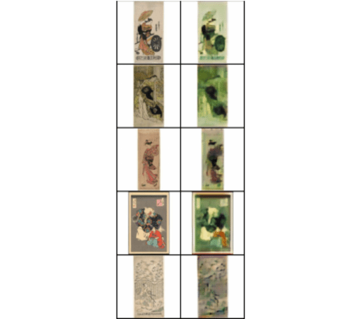
As you can see, the VQ-VAE does pretty well on reconstruction, which means that we were able to learn a representative set of embedding vectors with which to model our dataset.

For completeness, let’s also compare the learned prior outputs to outputs from the uniform prior over training. We’re just plotting the batches we generated from our earlier code.

comp-prior

As you can see, the uniform prior is insufficient to accurately capture the categorical distribution of the latent space, resulting in images with no discernible features (right) as compared to the learned prior (left). It’s likely possible to improve the generated output of the VQ-VAE by using a more powerful model for the prior or just simply through training the model more, but for now our results are satisfactory.

Wrap-up

The VQ-VAE model is relatively simple to train in comparison to the VAE. There are much fewer hyper-parameters to experiment with, and training is generally more stable because of the simpler latent space representation. Even so, it’s possible that for your dataset the VQ-VAE is simply not good enough at image generation. The bottleneck in this case is usually the model used to generate the prior - algorithms like Stable Diffusion and the VQ-GAN have unique solutions to this that build up from the VQ-VAE (which I’ll discuss in future articles).

If you’ve made it this far, thank for reading through as always! We will return to the VQ-VAE in the future, but for now our work here is done. For the next part of this series, I’ll move into the realm of GANs and cover a particularly unique and recent improvement on them - the ProGAN.

If you’d like to check out the full code for this series, you can visit my public repository .