Introduction to Generative AI: Vision Series (3/3) - DDPM

---

Introduction

---

This is part three of a series on generative A.I. If you’d like to check out the other posts in the series, you can take a look here and here .

In this series, we’ve been dissecting some of the more popular algorithms used for image generation, such as Variational Autoencoders and Generative Adversarial Networks. This time, we’ll be tackling another very popular category of generative models - diffusion models .

Denoising Diffusion Probabilistic Models

---

Diffusion models, more formally known as Denoising Diffusion Probabilistic models (DDPMs), are a recent addition to the space of generative A.I. that have had massive consequences on the field. Diffusion models are the backbone behind models like Stable Diffusion and DALL-E 2.

Before DDPMs, the primary image generation algorithms were based off the VAE or the GAN. GANs specialize in creating highly realistic images but sometimes struggle to produce a wide range of images. VAEs have the opposite problem - it’s very easy to produce a wide range of images but its harder to get more realistic features with them.

Diffusion models are a sort of happy medium between the two - its possible to get highly diverse images while still preserving image quality. As such, they’re an incredibly hot topic of research right now.

Let’s see how they work!

Setup

---

Diffusion models are at their core, a type of latent variable model. We’ve covered these before, in my last two posts (here and here ), but this time we’re going to do something a little different.

Let’s start with some input vector $\mathbf{x}_0$ that is sampled from the true data distribution $q(\mathbf{x})$ . We’re going to define our model $p_{\theta}(\mathbf{x}_0)$ in terms of $T$ different latent variables $\mathbf{x}_1 \dots \mathbf{x}_T$ instead of just one. If we define $\mathbf{x}_1 \dots \mathbf{x}_T$ to all be the same dimension as $\mathbf{x}_0$ , we can write
$$p_{\theta}(\mathbf{x}_0) = \int p_{\theta}(\mathbf{x}_{0:T}) \,d \mathbf{x}_{1:T}$$
We’re essentially taking an expectation of the value of the joint distribution $\mathbf{x}_{0:T}$ over another joint distribution $\mathbf{x}_{1:T}$ .

Reverse Process

---

We need something extra in order to compute the expression written above. A common setup in situations like this is a Markov chain , which is a formulation such that each $\mathbf{x}_i$ depends only on $\mathbf{x}_{i-1}$ . With this in mind, we can define distributions from $\mathbf{x}_0$ to $\mathbf{x}_T$ in a way such that we can tractably compute the joint distribution $p_{\theta}(\mathbf{x}_{0:T})$ . In this setting, the joint distribution $p_{\theta}(\mathbf{x}_{0:T})$ is known as the reverse process , and is defined as
$$p_{\theta}(\mathbf{x}_{0:T}) = p(\mathbf{x}_T) \prod_{t=1}^T p_{\theta}(\mathbf{x}_{t-1} | x_t)$$
where $p(\mathbf{x}_T) = \mathcal{N}(\mathbf{x}_T; \mathbf{0}, \mathbf{I})$ and
$$p_{\theta}(\mathbf{x}_{t-1} | \mathbf{x}_t) = \mathcal{N} (\mathbf{x}_{t-1}; \mu_{\theta}(\mathbf{x}_t, t), \Sigma_{\theta}(\mathbf{x}_t, t))$$
This last definition is the core of the Markov chain, and defines the Gaussian transitions that transform an input $\mathbf{x}_0$ throughout the chain into the output $\mathbf{x}_T$ .

Diffusion Process

---

The opposite of the reverse process is known as the diffusion process or forward process, written as $q(\mathbf{x}_{1:T} | \mathbf{x}_0)$ . This process is also fixed to a Markov chain, which gradually adds noise to the data $\mathbf{x}_0$ . We can further parameterize how much noise is added at each step using a variance schedule $\beta_1 \dots \beta_T$ . With this in mind, the diffusion process can be defined as
$$q(\mathbf{x}_{1:T} | \mathbf{x}_0) = \prod_{t=1}^T q(\mathbf{x}_t | \mathbf{x}_{t-1})$$
However, we need to define the transition $q(\mathbf{x}_t | \mathbf{x}_{t-1})$ in such a way that the added noise at each step doesn’t increase the overall variance. If we add noise for $T$ timesteps without scaling the input properly, we’ll end up with inputs in the range of $[-T, T]$ even if we started from an input of $\mathbf{x}_0 = \mathbf{0}$ . At any given timestep, we want $\mathbf{x}_t$ to have unit variance, so we have to manually scale the inputs $\mathbf{x}_{t-1}$ to satisfy this property.

Let’s call this scaling factor $a$ for now. At each step, we’ll also add the noise sampled from $\mathcal{N}(\mathbf{0}, \beta_t)$ according to our variance schedule. By the properties of the normal distribution, we can write this noise as $\sqrt{\beta_t}\epsilon_t$ where $\epsilon_t \sim \mathcal{N}(\mathbf{0}, \mathbf{I})$ . We can then write
$$\mathbf{x}_t = a\mathbf{x}_{t-1} + \sqrt{\beta_t}\epsilon_t$$
Let’s assume that $\mathbf{x}_{t-1}$ has unit variance (i.e. $\mathrm{Var}(\mathbf{x}_{t-1}) = 1$ ). By the properties of variance (refresher if you need it), you can then write $$\mathrm{Var}(\mathbf{x}_t) = a^2 + \beta_t$$
We’re going to force $\mathrm{Var}(\mathbf{x}_t) = 1$ , so if we solve this for $a$ , we’ll get $a = \sqrt{1 - \beta_t}$ . Therefore, we know that
$$\mathbf{x}_t = \sqrt{1 - \beta_t}\mathbf{x}_{t-1} + \sqrt{\beta_t}\epsilon_t$$
I won’t do a full proof by induction here, but what we did above works for every $t$ assuming that we scale the input $\mathbf{x}_0$ to also have unit variance. From this, we can then write
$$q(\mathbf{x}_t | \mathbf{x}_{t-1}) = \mathcal{N} (\mathbf{x}_t; \sqrt{1- \beta_t}\mathbf{x}_{t-1}, \beta_t\mathbf{I})$$

Arbitrary Sampling

---

One extra nice thing about this formulation above is that we can derive a closed form for $q(\mathbf{x}_t | \mathbf{x}_0)$ for any arbitrary $t$ . Let’s do that really quick - we’ll rewrite $\mathbf{x}_{t-1}$ in terms of $\mathbf{x}_{t-2}$ to start
$$\begin{align*} \mathbf{x}_{t} &= \sqrt{1 - \beta_t}\mathbf{x}_{t-1} + \sqrt{\beta_t}\epsilon_t\\ &= \sqrt{1 - \beta_t}(\sqrt{1 - \beta_{t-1}}\mathbf{x}_{t-2} + \sqrt{\beta_{t-1}}\epsilon_{t-1}) + \sqrt{\beta_t}\epsilon_t\\ &= \sqrt{1 - \beta_t}\sqrt{1 - \beta_{t-1}}\mathbf{x}_{t-2} + \sqrt{1 - \beta_t}\sqrt{\beta_{t-1}}\epsilon_{t-1} + \sqrt{\beta_t}\epsilon_t\\ \end{align*}$$
The last two terms here are Gaussian distributions with mean $\mathbf{0}$ , which means we can merge them as follows
$$\begin{align*} \sqrt{1 - \beta_t}\sqrt{\beta_{t-1}}\epsilon_{t-1} + \sqrt{\beta_t}\epsilon_t &= \sqrt{(1- \beta_t)\beta_{t-1}+\beta_t}\bar{\epsilon}_t \\ &= \sqrt{\beta_t + \beta_{t-1} - \beta_t\beta_{t-1}} \bar{\epsilon}_t\\ &= \sqrt{1 - (1 - \beta_t)(1 - \beta_{t-1})} \bar{\epsilon}_t \end{align*}$$
where we’ve reparameterized with $\bar{\epsilon}_t \sim \mathcal{N}(\mathbf{0}, \mathbf{I})$ . Let’s define $\alpha_t = 1 - \beta_t$ to make this a bit easier to look at. Going back to what we had earlier, this means
$$\begin{align*} \mathbf{x}_{t} &= \sqrt{\alpha_t}\mathbf{x}_{t-1} + \sqrt{1 - \alpha_t}\epsilon_t\\ &= \sqrt{\alpha_t\alpha_{t-1}}\mathbf{x}_{t-2} + \sqrt{1 - \alpha_t\alpha_{t-1}}\bar{\epsilon}_t\\ &\dots\\ &= \sqrt{\alpha_t\alpha_{t-1}\dots}\mathbf{x}_{0} + \sqrt{1 - \alpha_t\alpha_{t-1}\dots}\bar{\epsilon}_t \end{align*}$$
We can continue this calculation all the way to $\mathbf{x}_0$ . If we also define $\bar{\alpha}_t = \prod_{s=1}^t \alpha_s$ , we can then write
$$\mathbf{x}_t = \sqrt{\bar{\alpha}_t}\mathbf{x}_0 + \sqrt{1 - \bar{\alpha}_t}\bar{\epsilon}_t$$ and therefore
$$q(\mathbf{x}_t | \mathbf{x}_{0}) = \mathcal{N} (\mathbf{x}_t; \sqrt{\bar{\alpha}_t}\mathbf{x}_{0}, (1 - \bar{\alpha}_t)\mathbf{I})$$

This means that we can quickly sample from the posterior at any timestep $t$ without having to actually run through the full Markov chain, which is really nice for training.

Objective

---

As is the case for most latent variable models, we’d like to minimize the Kullback-Leibler divergence between our approximate posterior $q(\mathbf{x}_{1:T}| \mathbf{x}_0)$ and the true posterior $p_\theta(\mathbf{x}_{1:T} | \mathbf{x}_0)$ . We’ve derived this before (see my first article ), and it turns out that minimizing the Kullback-Leibler divergence for this setting is the same as maximizing the ELBO (evidence lower bound). We have that
$$\log p_{\theta}(\mathbf{x}) \geq \mathbb{E}_{q}\left[\log \frac{p_{\theta}(\mathbf{x}_{0:T})}{q(\mathbf{x}_{1:T} | \mathbf{x}_0)}\right]$$
where we want to maximize the right hand term. For the diffusion model, we can take this a little further using the definitions of our joint distributions from above, and write an objective $L$ to minimize as
$$\begin{align*} L &= -\mathbb{E}_{q}\left[\log \frac{p_{\theta}(\mathbf{x}_{0:T})}{q(\mathbf{x}_{1:T} | \mathbf{x}_0)}\right]\\ &= -\mathbb{E}_{q}\left[\log p_{\theta}(\mathbf{x}_{0:T}) - \log q(\mathbf{x}_{1:T} | \mathbf{x}_0)\right]\\ &= -\mathbb{E}_{q}\left[\log (p(\mathbf{x}_T) \prod_{t=1}^T p_{\theta}(\mathbf{x}_{t-1} | \mathbf{x}_t)) - \log \prod_{t=1}^T q(\mathbf{x}_t | \mathbf{x}_{t-1})\right]\\ &= \mathbb{E}_{q}\left[-\log p(\mathbf{x}_T) - \sum_{t=1}^T \log p_{\theta}(\mathbf{x}_{t-1} | \mathbf{x}_t) + \sum_{t=1}^T \log q(\mathbf{x}_t | \mathbf{x}_{t-1})\right]\\ &= \mathbb{E}_{q}\left[-\log p(\mathbf{x}_T) - \sum_{t=1}^T \log \frac{p_{\theta}(\mathbf{x}_{t-1} | \mathbf{x}_t)}{q(\mathbf{x}_t | \mathbf{x}_{t-1})} \right] \end{align*}$$

This formulation is nicer because we don’t have to compute the full joint distributions. However, there’s still an issue with this formulation - similar to the objective in the VAE, it has way too much variance to be useful as a training signal. The derivation for this next bit is super long (the original paper that introduced diffusion models goes into it in depth), but the tldr is that you can rewrite $L$ as follows

$$\begin{align*} L_0 &= \log p_{\theta}(\mathbf{x}_0 | \mathbf{x}_1)\\ L_{t-1} &= D_{KL} (q(\mathbf{x}_{t-1} | \mathbf{x}_t, \mathbf{x}_0) \parallel p_{\theta}(\mathbf{x}_{t-1} | \mathbf{x}_t))\\ L_T &= D_{KL} (q(\mathbf{x}_T | \mathbf{x}_0) \parallel p(\mathbf{x}_t))\\ L &= \mathbb{E}_q \left[L_T + \sum_{t=1}^T L_{t-1} - L_0 \right] \end{align*}$$
We can ignore $L_T$ when training since it is constant. Therefore, we only have to ensure that $L_0$ and $L_{t-1}$ are tractable terms during training. The original paper defines a discrete decoder for $L_0$ , but since it’s not as important for the implementation we’ll focus on $L_{t-1}$ .

Loss Tractability

---

In my previous articles, I’ve discussed the statistical fact that the Kullback-Liebler divergence has a closed form formula, which ensures that computing it results in less variance than a Monte Carlo estimate. We already have an expression for $p_{\theta}(\mathbf{x}_{t-1} | \mathbf{x}_t)$ from above, but we need to find a nice way to express $q(\mathbf{x}_{t-1} | \mathbf{x}_t, \mathbf{x}_0)$ for the computation of $L_{t-1}$ .

Let’s start with using Bayes’ Rule to rewrite $q(\mathbf{x}_{t-1} | \mathbf{x}_t, \mathbf{x}_0)$ and then simplify.

$$\begin{align*} q(\mathbf{x}_{t-1} | \mathbf{x}_t, \mathbf{x}_0) &= q(\mathbf{x}_{t} | \mathbf{x}_{t-1}, \mathbf{x}_0) \frac{q(\mathbf{x}_{t-1} | \mathbf{x}_0)}{q(\mathbf{x}_{t} | \mathbf{x}_0)}\\ \end{align*}$$
These terms can be expressed as Gaussian distributions using the expressions we’ve already derived above as follows.
$$\begin{align*} q(\mathbf{x}_{t} | \mathbf{x}_{t-1}, \mathbf{x}_0) &= \mathcal{N} (\mathbf{x}_t; \sqrt{\alpha_t}\mathbf{x}_{t-1}, \beta_t\mathbf{I}) \\ q(\mathbf{x}_{t} | \mathbf{x}_{t-1}, \mathbf{x}_0) &\propto \exp \left(-\frac{1}{2} \frac{(\mathbf{x}_t - \sqrt{\alpha_t}\mathbf{x}_{t-1})^2}{\beta_t}\right)\\ \\ q(\mathbf{x}_{t-1} | \mathbf{x}_0) &= \mathcal{N} (\mathbf{x}_{t-1}; \sqrt{\bar{\alpha}_{t-1}}\mathbf{x}_{0}, (1 - \bar{\alpha}_{t-1})\mathbf{I}) \\ q(\mathbf{x}_{t-1} | \mathbf{x}_0) &\propto \exp \left(-\frac{1}{2} \frac{(\mathbf{x}_{t-1} - \sqrt{\bar{\alpha}_{t-1}}\mathbf{x}_0)^2}{1 - \bar{\alpha}_{t-1}}\right)\\ \\ q(\mathbf{x}_{t} | \mathbf{x}_0) &= \mathcal{N} (\mathbf{x}_{t}; \sqrt{\bar{\alpha}_{t}}\mathbf{x}_{0}, (1 - \bar{\alpha}_{t})\mathbf{I}) \\ q(\mathbf{x}_{t} | \mathbf{x}_0) &\propto \exp \left(-\frac{1}{2} \frac{(\mathbf{x}_{t} - \sqrt{\bar{\alpha}_{t}}\mathbf{x}_0)^2}{1 - \bar{\alpha}_{t}}\right)\\ \end{align*}$$
So we can rewrite $q(\mathbf{x}_{t-1} | \mathbf{x}_t, \mathbf{x}_0)$ as $\propto \exp (-\frac{1}{2} f(\mathbf{x}_{t-1}))$ where
$$\begin{align*} f(\mathbf{x}_{t-1}) &= \frac{(\mathbf{x}_t - \sqrt{\alpha_t}\mathbf{x}_{t-1})^2}{\beta_t} + \frac{(\mathbf{x}_{t-1} - \sqrt{\bar{\alpha}_{t-1}}\mathbf{x}_0)^2}{1 - \bar{\alpha}_{t-1}} - \frac{(\mathbf{x}_{t} - \sqrt{\bar{\alpha}_{t}}\mathbf{x}_0)^2}{1 - \bar{\alpha}_{t}}\\ &= \frac{\mathbf{x}_t^2 - 2\sqrt{\alpha_t}\mathbf{x}_{t}\mathbf{x}_{t-1} + \alpha_t\mathbf{x}_{t-1}^2}{\beta_t} + \frac{\mathbf{x}_{t-1}^2 - 2\sqrt{\bar{\alpha}_{t-1}}\mathbf{x}_{t-1}\mathbf{x}_0 + \bar{\alpha}_{t-1}\mathbf{x}_0^2}{1 - \bar{\alpha}_{t-1}} - \frac{\mathbf{x}_{t}^2 - \sqrt{\bar{\alpha}_{t}}\mathbf{x}_{t}\mathbf{x}_0 + \bar{\alpha}_{t}\mathbf{x}_0^2}{1 - \bar{\alpha}_{t}}\\ &= \left(\frac{\alpha_t}{\beta_t} + \frac{1}{1 - \bar{\alpha}_{t-1}}\right)\mathbf{x}_{t-1}^2 - \left(\frac{2\sqrt{\alpha_t}\mathbf{x}_t}{\beta_t} + \frac{2\sqrt{\bar{\alpha}_{t-1}}\mathbf{x}_0}{1 - \bar{\alpha}_{t-1}} \right) \mathbf{x}_{t-1} + C(\mathbf{x}_t, \mathbf{x}_0) \end{align*}$$
where we’ve collected terms that don’t depend on $\mathbf{x}_{t-1}$ into $C(\mathbf{x}_t, \mathbf{x}_0)$ . We’ve done the regrouping of terms in this way so that the final distribution can be written as another Gaussian distribution; if we let
$$\begin{align*} \tilde{\beta}_t &= \frac{1}{\left(\frac{\alpha_t}{\beta_t} + \frac{1}{1 - \bar{\alpha}_{t-1}}\right)} = \frac{1}{\left(\frac{\alpha_t - \alpha_t\bar{\alpha}_{t-1} + \beta_t}{\beta_t(1 - \bar{\alpha}_{t-1})} \right)} \\ &= \frac{1 - \bar{\alpha}_{t-1}}{(1 - \beta_t) -\bar{\alpha}_{t} + \beta_t}\beta_t = \frac{1 - \bar{\alpha}_{t-1}}{1 - \bar{\alpha}_{t}}\beta_t \end{align*}$$
we can then write
$$\begin{align*} \tilde{\mu}_t(\mathbf{x}_t, \mathbf{x}_0) &= \left(\frac{\sqrt{\alpha_t}\mathbf{x}_t}{\beta_t} + \frac{\sqrt{\bar{\alpha}_{t-1}}\mathbf{x}_0}{1 - \bar{\alpha}_{t-1}} \right) \tilde{\beta}_t\\ &= \left(\frac{\sqrt{\alpha_t}\mathbf{x}_t}{\beta_t} + \frac{\sqrt{\bar{\alpha}_{t-1}}\mathbf{x}_0}{1 - \bar{\alpha}_{t-1}} \right) \frac{1 - \bar{\alpha}_{t-1}}{1 - \bar{\alpha}_{t}}\beta_t\\ &= \frac{\sqrt{\alpha_t}(1 - \bar{\alpha}_{t-1})}{1 - \bar{\alpha}_{t}}\mathbf{x}_t + \frac{\sqrt{\bar{\alpha}_{t-1}}\beta_t}{1 - \bar{\alpha}_{t}} \mathbf{x}_0 \end{align*}$$
and therefore we have
$$q(\mathbf{x}_{t-1} | \mathbf{x}_t, \mathbf{x}_0) = \mathcal{N} \left( \mathbf{x}_{t-1}; \tilde{\mu}_t(\mathbf{x}_t, \mathbf{x}_0), \tilde{\beta}_t\mathbf{I} \right)$$

Objective Reparameterization

---

With this above expression in hand, let’s return to the original loss objective. We’ll handle $L_0$ separately so looking at $L_{t-1}$ , we have the Kullback-Leibler divergence between $q(\mathbf{x}_{t-1} | \mathbf{x}_t, \mathbf{x}_0) = \mathcal{N} \left( \mathbf{x}_{t-1}; \tilde{\mu}_t(\mathbf{x}_t, \mathbf{x}_0), \tilde{\beta}_t\mathbf{I} \right)$ and $p_{\theta}(\mathbf{x}_{t-1} | \mathbf{x}_t) = \mathcal{N} (\mathbf{x}_{t-1}; \mu_{\theta}(\mathbf{x}_t, t), \Sigma_{\theta}(\mathbf{x}_t, t))$ .

In the original paper, the posterior variance $\Sigma_{\theta}(\mathbf{x}_t, t)$ is fixed to $\sigma_t^2\mathbf{I}$ where $\sigma_t^2 = \beta_t$ for simplicity. Now, because of the fact that both $q(\mathbf{x}_{t-1} | \mathbf{x}_t, \mathbf{x}_0)$ and $p_{\theta}(\mathbf{x}_{t-1} | \mathbf{x}_t)$ are Gaussian distributions, we can rewrite the expression as follows
$$L_{t-1} = \mathbb{E}_q \left[\frac{1}{2\sigma_t^2} \lVert \tilde{\mu}_t(\mathbf{x}_t, \mathbf{x}_0) - \mu_{\theta}(\mathbf{x}_t, t) \rVert ^2 \right] + C$$ where $C$ is a constant that does not depend on $\theta$ .

The most straightforward implementation using the objective above would be to predict the forward process posterior mean $\tilde{\mu}_t$ with $\mu_\theta$ . However, let’s bring back the property we derived earlier for the forward diffusion process. We know that $\mathbf{x}_t = \sqrt{\bar{\alpha}_t}\mathbf{x}_0 + \sqrt{1 - \bar{\alpha}_t}\epsilon$ where $\epsilon \sim \mathcal{N}(\mathbf{0}, \mathbf{I})$ , so we can rewrite $\mathbf{x}_0 = \frac{1}{\sqrt{\bar{\alpha}_t}} \left(\mathbf{x}_t - \sqrt{1 - \bar{\alpha}_t}\epsilon \right)$ . Then, we have
$$\begin{align*} \tilde{\mu}_t(\mathbf{x}_t, \mathbf{x}_0) &= \frac{\sqrt{\alpha_t}(1 - \bar{\alpha}_{t-1})}{1 - \bar{\alpha}_{t}}\mathbf{x}_t + \frac{\sqrt{\bar{\alpha}_{t-1}}\beta_t}{1 - \bar{\alpha}_{t}} \mathbf{x}_0 \\ \tilde{\mu}_t(\mathbf{x}_t, t) &= \frac{\sqrt{\alpha_t}(1 - \bar{\alpha}_{t-1})}{1 - \bar{\alpha}_{t}}\mathbf{x}_t + \frac{\sqrt{\bar{\alpha}_{t-1}}\beta_t}{1 - \bar{\alpha}_{t}} \frac{1}{\sqrt{\bar{\alpha}_t}} \left(\mathbf{x}_t - \sqrt{1 - \bar{\alpha}_t}\epsilon \right)\\ &= \frac{1}{\sqrt{\alpha_t}}\mathbf{x}_t - \frac{\beta_t}{\sqrt{1 - \bar{\alpha}_t}\sqrt{\alpha_t}} \epsilon_t \\ &= \frac{1}{\sqrt{\alpha_t}}\left( \mathbf{x}_t - \frac{\beta_t}{\sqrt{1 - \bar{\alpha}_t}} \epsilon\right) \\ \end{align*}$$
Here, we notice that $\mu_\theta$ must predict $\frac{1}{\sqrt{\alpha_t}}\left( \mathbf{x}_t - \frac{\beta_t}{\sqrt{1 - \bar{\alpha}_t}} \epsilon \right)$ given $\mathbf{x}_t$ . However, since we have $\mathbf{x}_t$ as an input for $\mu_\theta$ , we can just explicitly define the model to compute this quantity using the inputs given
$$\mu_\theta(\mathbf{x}_t, t) = \frac{1}{\sqrt{\alpha_t}}\left( \mathbf{x}_t - \frac{\beta_t}{\sqrt{1 - \bar{\alpha}_t}} \epsilon_\theta(\mathbf{x}_t, t) \right)$$
where we train a model $\epsilon_\theta(\mathbf{x}_t, t)$ to predict the added noise at step $t$ . With this formulation, the sampling procedure
$$\mathbf{x}_{t-1} \sim p_{\theta}(\mathbf{x}_{t-1} | \mathbf{x}_t) = \mathcal{N} (\mathbf{x}_{t-1}; \mu_{\theta}(\mathbf{x}_t, t), \sigma_t^2\mathbf{I})$$
becomes much simpler
$$\mathbf{x}_{t-1} = \frac{1}{\sqrt{\alpha_t}}\left( \mathbf{x}_t - \frac{\beta_t}{\sqrt{1 - \bar{\alpha}_t}} \epsilon_\theta(\mathbf{x}_t, t) \right) + \sigma_t \mathbf{z}$$
where $\mathbf{z} \sim \mathcal{N(\mathbf{0}, \mathbf{I})}$ . This is a very similar trick to the one used in the VAE - we’re basically moving the noise out of the actual model and into a small random variable that we sample at inference time.

With this new parameterization, the original objective also becomes a bit simpler.
$$\begin{align*} L_{t-1} - C &= \mathbb{E}_{x_0, \epsilon} \left[\frac{1}{2\sigma_t^2} \lVert \tilde{\mu}_t(\mathbf{x}_t, t) - \mu_{\theta}(\mathbf{x}_t, t) \rVert ^2 \right]\\ &= \mathbb{E}_{x_0, \epsilon} \left[\frac{\beta_t^2}{2\sigma_t^2\alpha_t(1 - \bar{\alpha}_t)} \Big\lVert \epsilon - \epsilon_\theta(\mathbf{x}_t, t) \Big\rVert ^2 \right]\\ \end{align*}$$
where we can also compute the $\mathbf{x}_t$ input for $\epsilon_\theta$ as $\mathbf{x}_t = \sqrt{\bar{\alpha}_t}\mathbf{x}_0 + \sqrt{1 - \bar{\alpha}_t}\epsilon$ . Both parameterizations from above are equally valid, but it’s usually more effective to train for $\epsilon_\theta$ in practice. The authors also derived a simplified version of the above objective, where we remove the leading constant and sample $t$ uniformly from $1$ through $T$ as follows
$$L_{\text{simple}} = \mathbb{E}_{t, x_0, \epsilon} \left[ \lVert \epsilon - \epsilon_\theta(\mathbf{x}_t, t) \rVert ^2 \right]$$
This final objective is the one most often used in practice, and it’s what we’ll use for our implementation (finally ) in the following sections.

Implementation

---

With the theory out of the way, we can finally get around to implementing the model. The main structure of the neural network we’ll construct for $\epsilon_\theta(\mathbf{x}_t, t)$ is going to be a UNet, modeled off the famous PixelCNN .

UNets are common structures in computer vision that utilize a sort of encoder-decoder like architecture to return inputs of the same size as the original. In this case, this is very useful since we’d like the model $\epsilon_\theta(\mathbf{x}_t, t)$ to predict the noise we added originally to get to $\mathbf{x}_t$ , which will be the same size as it.

It’s also very common to include something called skip connections or residual connections in UNets, which are just essentially connections between layers where you add the output of one layer back into the input of another layer. This is helpful for improving information flow through deep neural networks, since it preserves and reintroduces older features back into deeper stages of the network.

In the original paper, the authors found it useful to make some modifications to the PixelCNN backbone that improved the overall performance for the purposes of diffusion. We’ll go through those changes one by one in the following sections, which will turn the baseline UNet into a complete NoiseNet implementation.

Before we make any of the actual code, let's quickly implement a few helper functions.

        
def extract(t):
    # unsqueeze Tensor to have 4 dimensions
    for _ in range(4 - len(t.shape)):
        t = torch.unsqueeze(t, -1)
    return t

def scale_0_1(image):
    # scale any Tensor to 0 to 1
    image = image - torch.amin(image, dim=(2, 3), keepdim=True)
    return image / torch.amax(image, dim=(2, 3), keepdim=True)

def scale_minus1_1(image):
    # scale 0 to 1 Tensor to -1 to 1
    return image * 2 - 1
    

Attention

---

We need to implement a Attention layer (which is also from the attention paper) for our NoiseNet . This block helps focus the model on relevant aspects of the input image in the noise prediction process. The authors utilized this module at lower feature depths to improve the model’s performance in conjunction with the time inputs $t$ .

I will cover attention in more detail in a later post, so for now I’ll simply include the code implementing this module. If you’d like to learn more about attention, I found this tutorial very helpful.

        
class Attention(nn.Module):
    def __init__(self, dim, heads=4, dim_head=32):
        super().__init__()
        self.scale = dim_head ** -0.5
        self.heads = heads
        self.dim_head = dim_head
        self.hidden_dim = dim_head * heads
        self.norm = nn.GroupNorm(1, dim)
        self.to_qkv = nn.Conv2d(dim, self.hidden_dim * 3, 1, bias=False)
        self.to_out = nn.Conv2d(self.hidden_dim, dim, 1)

    def forward(self, x):
        b, c, h, w = x.shape
        x = self.norm(x)
        qkv = self.to_qkv(x).chunk(3, dim = 1)
        q, k, v = map(lambda t: t.view(b, self.heads, self.dim_head, h * w), qkv)

        q = q * self.scale
        sim = torch.einsum("b h c i, b h c j -> b h i j", q, k)
        sim = sim - sim.amax(dim=-1, keepdim=True).detach()
        attention = sim.softmax(dim=-1)

        out = torch.einsum("b h i j, b h c j -> b h i c", attention, v)
        out = out.permute(0, 1, 3, 2).reshape((b, self.hidden_dim, h, w))
        return self.to_out(out)
    

Upblock, Midblock, Downblock

---

The backbone of the network will be composed of blocks, which we'll call Upblock, Midblock, and Downblock. These blocks encapsulate the logic for the encoder and decoder parts of the UNetrespectively. Since they'll implement residual connections, they'll also require specialized .forward methods. I've included the code for each in its entirely below - we'll go into the inner details in subsequent sections.

One important thing to note is that these blocks return multiple outputs, so that we can implement skip connections in the main NoiseNet. In particular, Upblock has a specialized residual input that we use like a stack for our residual connections. Downblock returns these residuals, so we'll have to use some special logic in the overall NoiseNet to tie these blocks together.

        
class UpBlock(nn.Module):
    def __init__(self, dim_in, dim_out, dim_time, attn=False, upsample=True):
        super().__init__()

        self.block1 = ResnetBlock(dim_out + dim_in, dim_out, dim_time)
        self.block2 = ResnetBlock(dim_out + dim_in, dim_out, dim_time)
        self.attn = Attention(dim_out) if attn else nn.Identity()
        self.us = Upsample(dim_out, dim_in) if upsample else nn.Conv2d(dim_out, dim_in, 3, padding=1) 

    def forward(self, x, t, r):
        x = torch.cat((x, r.pop()), dim=1)
        x = self.block1(x, t)
        x = torch.cat((x, r.pop()), dim=1)
        x = self.block2(x, t)
        x = self.attn(x)
        x = self.us(x)
        return x 

class MidBlock(nn.Module):
    def __init__(self, dim, dim_time):
        super().__init__()

        self.conv1 = ResnetBlock(dim, dim, dim_time)
        self.attn = Attention(dim)
        self.conv2 = ResnetBlock(dim, dim, dim_time)

    def forward(self, x, t):
        x = self.conv1(x, t)
        x = self.attn(x)
        x = self.conv2(x, t)
        return x
    
class DownBlock(nn.Module):
    def __init__(self, dim_in, dim_out, dim_time, attn=False, downsample=True):
        super().__init__()

        self.block1 = ResnetBlock(dim_in, dim_in, dim_time)
        self.block2 = ResnetBlock(dim_in, dim_in, dim_time)
        self.attn = Attention(dim_in) if attn else nn.Identity()
        self.ds = Downsample(dim_in, dim_out) if downsample else nn.Conv2d(dim_in, dim_out, 3, padding=1)

    def forward(self, x, t):
        residuals = []
        x = self.block1(x, t)
        residuals.append(x.clone())
        x = self.block2(x, t)
        x = self.attn(x)
        residuals.append(x.clone())
        x = self.ds(x)
        return x, residuals
    

ResNetBlock

---

The core block in the Upblock Midblock and Downblock is a ResNetBlock . This module takes in a time input as well as the image feature input and transforms it into the next stage of features. An important note here is that by implementing the block in this fashion, the DDPM allows for time inputs to be included at every stage in the diffusion process.

        
class ResnetBlock(nn.Module):
    def __init__(self, in_channels, out_channels, time_embedding_dim):
        super().__init__()

        self.time_fc = nn.Linear(time_embedding_dim, in_channels)
        self.conv1 = ConvBlock(in_channels, out_channels) 
        self.conv2 = ConvBlock(out_channels, out_channels) 

        self.conv_res = (
            nn.Conv2d(in_channels, out_channels, 1)
            if in_channels != out_channels else nn.Identity()
        )
    

Each ResNet block also utilizes residual connections internally, which require a specialized .forward method.

        
def forward(self, x, t):
    t_emb = self.time_fc(F.silu(t))[:, :, None, None]
    h = self.conv1(x + t_emb)
    h = self.conv2(h)
    r = self.conv_res(x)
    return h + r
    

ConvBlock

---

All of the above blocks utilize one component - the ConvBlock. This block simply packages a Conv2d operation with group normalization and an activiation function.

        
class ConvBlock(nn.Module):
    def __init__(self, in_channels, out_channels, groups=4):
        super().__init__()

        self.norm = nn.GroupNorm(groups, out_channels)
        self.conv = nn.Conv2d(in_channels, out_channels, 3, padding=1)

    def forward(self, x):
        x = self.conv(x)
        x = self.norm(x)
        return F.silu(x)
    

Upsample and Downsample

---

There’s not much theory behind these modules so I’ll keep it brief.

The Upsample block is implemented as a normal upsampling with the addition of a convolutional layer for feature extraction.

        
class Upsample(nn.Module):
    def __init__(self, in_channels, out_channels):
        super().__init__()

        self.model = nn.Sequential(
            nn.Upsample(scale_factor=2, mode='nearest'),
            nn.Conv2d(in_channels, out_channels, 3, padding=1)
        )

    def forward(self, x):
        return self.model(x)
    

The Downsample block is a bit more complicated. Essentially, we’re taking features from the image dimensions and moving them to the channel dimensions as a form of downsampling. Again, there’s also an added convolutional layer for feature extraction.

        
class Downsample(nn.Module):
    def __init__(self, in_channels, out_channels):
        super().__init__()

        self.model = nn.Sequential(
            Rearrange("b c (h p1) (w p2) -> b (c p1 p2) h w", p1=2, p2=2),
            nn.Conv2d(in_channels * 4, out_channels, 1),
        )

    def forward(self, x):
        return self.model(x)
    

Time Embedding

---

Finally, we need to implement an embedding layer for the input timestep t . This will convert the input $t$ from a single dimensional input into a vector that can be better used by the model at each of the stages covered above. We’ll use another concept mentioned by the attention paper known as sinusoidal position embedding . I won’t go into the theory in detail here (I’ll cover it in a later post on the Transformer), so for our purposes the implementation is pretty simple.

        
class SinusoidalPosEmb(nn.Module):
    def __init__(self, dim, device, theta=10000):
        super().__init__()
        self.dim = dim
        self.device = device
        self.theta = theta

    def forward(self, time):
        half_dim = self.dim // 2
        emb = math.log(self.theta) / (half_dim - 1)
        emb = torch.exp(torch.arange(half_dim, device=self.device) * -emb)
        emb = time[:, None] * emb[None, :]
        emb = torch.cat((emb.sin(), emb.cos()), dim=-1)
        return emb
    

NoiseNet

---

With all the above components in place, we can construct the full noise prediction network. In the code below, we create the main blocks of the NoiseNet in a UNet-like structure.

        
class NoiseNet(nn.Module):
    def __init__(self, args, init_dim=64, dim_mults = [1, 2, 4, 8, 16], attn_resolutions = [16]):
        super(NoiseNet, self).__init__()

        self.args = args
        self.attn_resolutions = attn_resolutions
        self.input_conv = nn.Conv2d(args.channel_size, init_dim, 7, padding=3)

        num_resolutions = len(dim_mults)
        dims = [init_dim] + [init_dim * mult for mult in dim_mults]
        resolutions = [init_dim] + [int(args.dim * r) for r in torch.cumprod(torch.ones(num_resolutions) * 0.5, dim=0).tolist()]
        in_out_res = list(enumerate(zip(dims[:-1], dims[1:], resolutions)))

        self.downs = nn.ModuleList([])
        for i, (dim_in, dim_out, res) in in_out_res:
            downsample = (i < (num_resolutions - 1))
            attn = (res in attn_resolutions)

            self.downs.append(
                DownBlock(dim_in, dim_out, dim_time, attn, downsample)
            )

        dim_mid = dims[-1]
        self.mid = MidBlock(dim_mid, dim_time)

        self.ups = nn.ModuleList([])
        for i, (dim_in, dim_out, res) in reversed((in_out_res)):
            upsample = (i > 0)
            attn = (res in attn_resolutions)

            self.ups.append(
                UpBlock(dim_in, dim_out, dim_time, attn, upsample)
            )

        self.output_res = ResnetBlock(init_dim * 2, init_dim, dim_time)
        self.output_conv = nn.Conv2d(init_dim, args.channel_size, 1)
    

We’ll also create a small network to embed the time input as a vector.

        
dim_time = dim * 4
self.time_embedding = nn.Sequential(
    SinusoidalPosEmb(dim = dim, device=device),
    nn.Linear(dim, dim_time),
    nn.GELU(),
    nn.Linear(dim_time, dim_time)
)
    

Since we’re implementing residual connections in the NoiseNet, we’ll also require some specialized code in the forward() method for the module. The way a residual connection is implemented here is to just make a copy of the input at the start of the connection and then add that to the end of the connection in forward() .

        
def forward(self, x, t):
    t = self.time_embedding(t)
    x = self.input_conv(x)
    res_stack = [x.clone()]

    for down in self.downs:
        x, residuals = down(x, t)
        res_stack += residuals

    x = self.mid(x, t)

    for up in self.ups:
        x = up(x, t, res_stack)

    x = torch.cat((x, res_stack.pop()), dim=1)
    x = self.output_res(x, t)
    x = self.output_conv(x)
    return x
    

Sampling and Noise Addition

---

To make things a bit easier, we’re going to wrap all these components up into one module - a DenoisingDiffusionModel.

In addition to the NoiseNet , this module will also store the buffers for $\beta, \alpha$ , and all the other variables we need for the implementations of the noise addition and sampling procedures.

        
class DenoisingDiffusionModel(nn.Module):
    def __init__(self, device):
        super(DenoisingDiffusionModel, self).__init__()

        self.device = device

        self.noise_net = NoiseNet(dim_mults=(1, 2, 4, 8, 16))

        T = torch.tensor(t).to(torch.float32)
        beta = torch.linspace(b_0, b_t, t, dtype=torch.float32, device=device)

        alpha = 1.0 - beta
        alpha_bar = torch.cumprod(alpha, dim=0)
        one_minus_alpha_bar = 1.0 - alpha_bar

        sqrt_alpha = torch.sqrt(alpha)
        sqrt_alpha_bar = torch.sqrt(alpha_bar)
        sqrt_one_minus_alpha_bar = torch.sqrt(one_minus_alpha_bar)

        self.register_buffer("T", T)
        self.register_buffer("beta", beta)
        
        self.register_buffer("alpha", alpha)
        self.register_buffer("alpha_bar", alpha_bar)
        self.register_buffer("one_minus_alpha_bar", one_minus_alpha_bar)

        self.register_buffer("sqrt_alpha", sqrt_alpha)
        self.register_buffer("sqrt_alpha_bar", sqrt_alpha_bar)
        self.register_buffer("sqrt_one_minus_alpha_bar", sqrt_one_minus_alpha_bar)
    

We’ll also implement the noising and sampling procedures that we derived from above.

The noising procedure goes like this -
$$\mathbf{x_t} = \sqrt{\bar{\alpha}_t}\mathbf{x_0} + \sqrt{1 - \bar{\alpha}_t}\epsilon$$ which is implemented as

        
def _noise_t(self, x0, t):
    sqrt_alpha_bar = extract(self.sqrt_alpha_bar[t])
    sqrt_one_minus_alpha_bar = extract(self.sqrt_one_minus_alpha_bar[t])
    noise = torch.randn_like(x0, device=self.device)
    xt = sqrt_alpha_bar * x0 + sqrt_one_minus_alpha_bar * noise
    return xt, noise
    

The sampling procedure is a bit more complicated. Let’s first implement the sample method for a given timestep $t$ .
$$\mathbf{x_{t-1}} = \frac{1}{\sqrt{\alpha_t}} \left(\mathbf{x_{t}} - \frac{\beta_t}{\sqrt{1 - \bar{\alpha}_t}} \epsilon_{\theta}(\mathbf{x_{t}} , t)\right) + \sigma_t\mathbf{z}$$

        
def _get_sample_ts(self):
    T = self.T.int().item()
    ts = torch.linspace(0, T, steps=11)
    ts -= torch.ones_like(ts)
    ts[0] = 0.0
    return torch.round(ts)

@torch.inference_mode()
def _sample_t(self, xt, t):
    ts = torch.ones((len(xt), 1), dtype=torch.float32, device=self.device) * t
    beta = extract(self.beta[t])
    sqrt_alpha = extract(self.sqrt_alpha[t])
    sqrt_one_minus_alpha_bar = extract(self.sqrt_one_minus_alpha_bar[t])

    noise_pred = self.noise_net(xt, ts)
    xt_prev = (xt - noise_pred * beta / sqrt_one_minus_alpha_bar) / sqrt_alpha

    if t > 0:
        posterior_variance = beta ** 0.5
        xt_prev += posterior_variance * torch.randn_like(xt_prev, device=self.device)
    return xt_prev
    

The sampling procedure then just involves running the sample_t method across the timesteps in reverse order.

        
@torch.inference_mode()
def sample(self, shape):
    images_list = []
    xt = torch.randn(shape, device=self.device)
    T = self.T.int().item()
    sample_ts = self._get_sample_ts()

    for t in tqdm(reversed(range(0, T)), position=0):
        xt = self._sample_t(xt, t)
        if t in sample_ts:
            images_list.append(scale_0_1(xt).cpu())
    return images_list
    

We just need one final forward method to complete the code.

        
def forward(self, x):
    T = self.T.int().item()
    ts = torch.randint(T, (x.shape[0],), device=self.device)
    xt, noise = self._noise_t(x, ts)
    noise_hat = self.noise_net(xt, ts)
    return noise_hat, noise
    

And with that, we’re done with the code!

Generating Art

---

Now that we have the base network complete, lets put together a quick training loop and dataset to generate some new cool images!

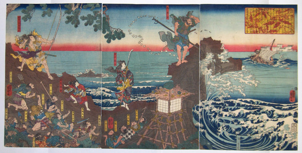
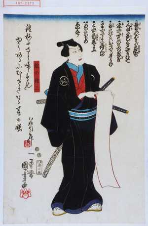
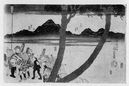
Many posts about DDPMs online use the MNIST dataset or the CelebA faces dataset; for this series, I’ll using more challenging datasets to better represent the difficulties of training these algorithms in the wild. As in my earlier post , all the experiments below use images from the Japanese Woodblock Print database .

Let’s try and generate images like the one above!

Again, I’ll skip the steps of defining the dataset and dataloader since they’re usually pretty simple and instead focus on the training loop. If you’d like to see that code, you can check out the full repo here .

Since we’ve already defined our other functions, the main training loop is also pretty simple. We just need to minimize the MSE between the actual noise and the predicted noise from our noise net over the samples in the training dataset. We’ll randomly sample timesteps $t$ throughout training - with enough batches we should reach good coverage over all $t$ from $1$ through $T$ .

        
ddpm = DenoisingDiffusionModel(device)
ddpm.to(device)
optimizer = optim.Adam(ddpm.parameters(), lr=lr)

losses = []

for epoch in range(n):

    progress_bar = tqdm(total=len(self.dataloader))
    progress_bar.set_description(f"Epoch {epoch}")

    for i, batch in enumerate(self.dataloader, 0):
        batch, _ = batch
        batch = batch.to(device)
        batch = scale_minus1_1(batch)

        optimizer.zero_grad()
        batch_noise_hat, batch_noise = ddpm(batch)
        loss = F.mse_loss(batch_noise_hat, batch_noise)
        loss.backward()
        optimizer.step()

        losses.append(loss.item())

        #############################
        ####   Metrics Tracking  ####
        #############################

        if i % 100 == 0:
            print(f'[%d/%d][%d/%d]\tloss: %.4f'
                % (epoch, n, i, len(self.dataloader), loss.item()))
            
        progress_bar.update(1)
            
    if epoch == 0:
        plot_batch(scale_0_1(batch), self.progress_dir + f"train_example")

    fake = ddpm.sample(batch.shape)[-1]
    plot_batch(scale_0_1(fake), self.progress_dir + f"epoch:{epoch:04d}")
    

For training, I ran the procedure for n = 10 epochs using a constant learning rate of 2e-5 and T = 1000 . Diffusion models often take a long time to train due to the amount of data required, as well as the time taken to run the sampling procedure for intermittent results, so be ready to be patient.

Once we’ve completed training we can take a look at our generated images. As per usual, I've included images from the dataset that I feel look similar.

The images generated here are pretty decent! Even with an unclean, relatively limited dataset (roughly 200K images) in the context of diffusion models, our model is able to generate images with some surprising details. You can even see some attempts at calligraphy in the generated images above, proof that the model is capable of learning fine details from the dataset. We can see clear similarities between some of the dataset images and the generated art above, but the diffusion model still does have some way to go to get to real artwork.

Let’s also take a look at how the diffusion model improves on the same batch of latent inputs (fixed_latent ) from above throughout training.

For completeness, let’s also visualize the progressive denoising of a generated image. The code for this just involves storing the generated images every 100 timesteps for display. Click the animation again if you'd like to restart it.

Tips and Tricks

---

Training a diffusion model isn’t as difficult as some of the other algorithms we’ve looked at, but there are still some small, easy to implement tricks you can add to your implementation that can significantly improve the overall results.

1. Modify variance

   One quick trick is to replace the posterior variance $\sigma^2 = \beta_t$ in the sampling procedure with $\sigma^2 = \widetilde{\beta}_t = \frac{(1 - \bar{\alpha}_{t-1})}{1 - \bar{\alpha}_t}\beta_t$ . The authors of the paper say that both values end up producing similar results, but $\sigma^2 = \beta_t$ is more suitable for $\mathbf{x}_0 \sim \mathcal{N(\mathbf{0}, \mathbf{I}})$ while $\sigma^2 = \widetilde{\beta}_t$ is more suitable when $\mathbf{x}_0$ is deterministically set to one point. In code, its as simple as changing posterior_variance to

                   
   one_minus_alpha_bar_prev = self.one_minus_alpha_bar[t-1] if t >= 0 else torch.tensor(0.0)
   one_minus_alpha_bar = self.one_minus_alpha_bar[t]
   posterior_variance = beta * one_minus_alpha_bar_prev / one_minus_alpha_bar
               

2. Modify schedules

   In my implementation, I utilized a linear schedule over $\beta$ . In practice, some implementations utilize other schedules such as sigmoid, cosine or quadratic schedules. These schedules change what $\beta$ looks like over the timesteps $t$ . It’s hard to tell how this will affect the results ahead of time but it’s something to try.

   Another related tip to try is a different learning rate schedule. Usually, its easiest to keep the learning rate constant over training but sometimes other schedules like the ones I mentioned above can have a positive effect on training. Again, it’s hard to tell how this will affect the results ahead of time but it may be worth testing out.

3. Clipping in sampling procedure

   Another quick thing to try out would be replacing the sampling procedure with a version that uses clipping. The motivation here is that since we know $\mathbf{x}_0$ should be between $-1$ and $1$ , we can force the prediction $\widetilde{\mathbf{x}}_0$ to also be within this range when computing $\mathbf{x}_{t-1}$ . Instead of our original sampling procedure we would compute
   $$\mathbf{\widetilde{x}}_{0} = \frac{1}{\sqrt{\alpha_t}} \left(\mathbf{x}_{t} - \sqrt{1 - \bar{\alpha}_t}\epsilon_{\theta}(\mathbf{x}_{t} , t)\right)\\ \mathbf{x}_{t-1} = \frac{\sqrt{\bar{\alpha}_{t-1}}\beta_t }{1 - \bar{\alpha}_t} Clip_{-1}^{+1} (\mathbf{\widetilde{x}}_{0}) + \frac{\sqrt{\alpha_t}(1 - \bar{\alpha}_{t-1})}{1 - \bar{\alpha}_t}\mathbf{x}_t+ \sigma_t\mathbf{z}$$
   In code, this involves changing the sample_t method to

                   
   @torch.inference_mode()
   def _sample_t(self, xt, t):
       ts = torch.ones((len(xt), ), dtype=torch.float32, device=self.device) * t
       beta = extract(self.beta[t])
   
       sqrt_alpha = extract(self.sqrt_alpha[t])
       sqrt_alpha_bar = extract(self.sqrt_alpha_bar[t])
       sqrt_alpha_bar_prev = extract(self.sqrt_alpha_bar[t-1] if t >= 0 else torch.tensor(1.0))
   
       one_minus_alpha_bar = extract(self.one_minus_alpha_bar[t])
       one_minus_alpha_bar_prev = extract(self.one_minus_alpha_bar[t-1] if t >= 0 else torch.tensor(0.0))
       sqrt_one_minus_alpha_bar = extract(self.sqrt_one_minus_alpha_bar[t])
       
       x0_coeff = sqrt_alpha_bar_prev * beta / one_minus_alpha_bar
       xt_coeff = sqrt_alpha * one_minus_alpha_bar_prev / one_minus_alpha_bar
   
       #noise_pred = self.noise_net(xt, ts[:, None])
       noise_pred = self.noise_net(xt, ts.squeeze()).sample
       x0_pred = (xt - noise_pred * sqrt_one_minus_alpha_bar) / sqrt_alpha_bar
       x0_pred = torch.clamp(x0_pred, min=-1, max=1)
       xt_prev = x0_coeff * x0_pred + xt_coeff * xt
   
       if t > 0:
           posterior_variance = beta ** 0.5
           xt_prev += posterior_variance * torch.randn_like(xt, device=self.device)
       return xt_prev
               

4. Clipping gradient norm

   One nice thing a lot of official implementations do is clip the gradient norms before updating the model parameters. This prevents exploding gradients when you’re training the model and can help stabilize training in the long run. In PyTorch, this is very easy to add in the training loop

                   
   torch.nn.utils.clip_grad_norm_(ddpm.parameters(), 1.0)
               

The tricks above can be helpful, but with diffusion models the best solution is often simply more data and better data . While the math for deriving diffusion models gets quite complicated, as we have seen, the actual implementations are not difficult and the models are generally stable to train. This lends makes diffusion models well suited for simply throwing more data at if you want better results.

With this article, we’ve covered the main trifecta of vision algorithms in practice today and completed the Intro to Generative A.I.: Vision Series ! However, we’ve only really gone through the baseline algorithms in use today - we have yet to go over the many improvements and additions researchers have made upon the VAE, the GAN, and the DDPM.

With that in mind, my next article will start off something new - the Advanced Generative A.I.: Vision Series . This series will cover some more advanced models and go closer to the state of the art for image generation algorithms today. For the first article there, I’ll cover an interesting modification to the VAE (an old friend of ours ) - the vector quantized VAE, or VQ-VAE .

If you’d like to check out the full code for this series, you can visit my public repository .

---