Introduction to Generative AI: Vision Series (2/3) - GAN

---

Introduction

---

This is part two of a series on generative A.I. If you’d like to check out the first post in the series, you can take a look here.

In this series, I’ll be dissecting some of the more popular algorithms used for image generation, such as Variational Autoencoders, Generative Adversarial Networks, and Diffusion models. This time, we’ll be tackling Generative Adversarial Networks.

Generative Adversarial Networks

---

Originally proposed in 2014, the generative adversarial network (GAN) has become an immensely popular tool for image and data generation. GANs are known for their ability to generate fine details and model complex datasets. I’ll provide a rough overview of the paper, going through some of the math behind the GAN while skipping past some of the more technical details.

Setup

---

The core idea behind the GAN is to simultaneously train two models; the generator model will approximate a distribution $p_g(x)$ over some data $x$ , while the discriminator will attempt to predict, given an input $x$ , whether or not it comes from the data or $p_g(x)$ . A common analogy that’s used to describe this is like counterfeiters and police; the counterfeiters (generator) try and make fake money, while the police (discriminator) are constantly checking if the money is real or fake.

In more formal terms, we’ll define two models. The generator will be a function $G_{\theta_g}(z)$ that takes an input of random noise $z \sim p(z)$ and maps that noise to the data space. The discriminator will be a function $D_{\theta_d}(x)$ that’ll output a scalar value signifying the probability that $x$ came from $p_g(x)$ as opposed to the real data. In our scenario, we’ll also specify that both $D$ and $G$ are multilayer perceptrons or deep neural networks parameterized by $\theta_d$ and $\theta_g$ respectively.

Our main goal has two parts. First, we want to train $D$ to maximize the probability of assigning correct labels to both samples from $p_g$ and from the real dataset. Second, we want to minimize the probability that a sample from $G$ is detected as real. We can write this as a minimax game played by $G$ and $D$ with the value function $V(D, G)$ as follows
$$\min_G \max_D V(D, G) = \mathbb{E}_{x\sim p_{data}(x)} [\log D(x)] + \mathbb{E}_{z\sim p(z)} [ \log (1 - D(G(z)))]$$
The first term $\mathbb{E}_{x\sim p_{data}(x)} [\log D(x)]$ corresponds to maximizing the probability that the discriminator $D$ can correctly classify samples from the real dataset $p_{data}(x)$ . The second term $\mathbb{E}_{z\sim p(z)} [ \log (1 - D(G(z)))]$ is a bit more complicated; it corresponds to minimizing the probability that a sample $G(z)$ is detected as real, which requires using $D$ . This is where the adversarial nature of GANs come into play - $G$ and $D$ are essentially working against each other at the same time, respectively trying to minimize and maximize this term.

Theoretical Analysis

---

The setup above is pretty simple - however, we don’t really have any guarantees at the moment that $G$ and $D$ will be able to find a global optimum. This is true for minimax games in general, especially when dealing with complex functions like neural networks which are hard to analyze analytically. We also need to confirm whether or not a global optimum does actually exist, or whether the algorithm will continuously fluctuate between various equally valid states.

Let’s confirm the global optimum first. We can rewrite the objective above from the perspective of the discriminator $D$ . We want to maximize
$$\int_x p_{data}(x) \log D(x) \,dx+ \int_z p(z) \log (1 - D(G(z)) \,dz$$
I’ve rewritten the expectation as integrals using the idea that $\mathbb{E}_x[f(x)] = \int_x p(x) f(x) \,dx$ . We can simplify by removing the dependence on $z$ and $G(z)$ , instead replacing that with the generated distribution $p_g(x)$ .
$$\int_x p_{data}(x) \log D(x) \,dx+ \int_x p_{g}(x) \log (1 - D(x)) \,dx =\\ \int_x p_{data}(x) \log D(x) + p_{g}(x) \log (1 - D(x)) \,dx$$
Essentially, we’re trying to maximize $p_{data}(x) \log D(x) + p_{g}(x) \log (1 - D(x))$ for each $x$ . If we fix $x$ , we can treat $p_{data}(x)$ and $p_{g}(x)$ as constants ( $a$ and $b$ respectively). We can also replace $D(x)$ with a placeholder variable $y$ to make the following analysis a bit easier, making our equation $a \log y + b \log (1 - y)$ .

To find the stationary points of this function, we can take the derivative of this with respect to $y$ , set it to zero, and solve for $y$
$$\begin{align*} \frac{a}{y} - \frac{b}{1 - y} &= 0\\ \frac{a}{y} &= \frac{b}{1 - y}\\ a - ay &= by\\ a &= (a + b)y\\ y &= \frac{a}{a+b} \end{align*}$$
Therefore, replacing $a$ and $b$ with what we had earlier, for a fixed generator $G$ , the optimal discriminator $D$ for this minimax game is
$$D^*(x) = \frac{p_{data}(x)}{p_{data}(x) + p_{g}(x)}$$
Let’s use this to show that $p_g(x) = p_{data}(x)$ is optimal for $G$ in the full minimax game. First, since we assume a fixed $G$ and $D = D^*$ from earlier, we can rewrite $V(D, G)$ into a function that just describes the cost $C(G)$ of this fixed $G$ ,
$$C(G) = \mathbb{E}_{x\sim p_{data}(x)} \left[\log \frac{p_{data}(x)}{p_{data}(x) + p_{g}(x)} \right] + \mathbb{E}_{x\sim p_g(x)} \left[\log \frac{p_{g}(x)}{p_{data}(x) + p_{g}(x)}\right]$$
When $p_g(x) = p_{data}(x)$ , we have that $C(G) = \mathbb{E}_{x\sim p_{data}(x)}[\log \frac{1}{2}] + \mathbb{E}_{x\sim p_{g}(x)}[\log \frac{1}{2}] = -\log 4$ . To show that this is a global optimum, we can look at the difference between $C(G)$ and the following.
$$C(G) + \log 4 = \mathbb{E}_{x\sim p_{data}(x)} \left[\log \frac{p_{data}(x)}{p_{data}(x) + p_{g}(x)} \right] - \mathbb{E}_{x\sim p_{data}(x)}\left[\log \frac{1}{2}\right] + \\ \mathbb{E}_{x\sim p_g(x)} \left[\log \frac{p_{g}(x)}{p_{data}(x) + p_{g}(x)}\right] - \mathbb{E}_{x\sim p_{g}(x)}\left[\log \frac{1}{2}\right]$$
$$= \mathbb{E}_{x\sim p_{data}(x)} \left[\log \frac{2p_{data}(x)}{p_{data}(x) + p_{g}(x)} \right] + \mathbb{E}_{x\sim p_g(x)} \left[\log \frac{2p_{g}(x)}{p_{data}(x) + p_{g}(x)}\right]$$
Recall that the definition of the Kullback-Leibler divergence is $D_{KL}(p(x) || q(x)) = \mathbb{E}_{x \sim p(x)} \left[\log \frac{p(x)}{q(x)}\right]$ . We can see this pattern in the formula above, so let’s rewrite it as
$$C(G) = -\log 4 + D_{KL}\left( p_{data}(x) \Big\Vert \frac{p_{data}(x) + p_g(x)}{2}\right) \\ + D_{KL}\left( p_{g}(x) \Big\Vert \frac{p_{data}(x) + p_g(x)}{2}\right)$$
The Jenson-Shannon divergence is another measure that is essentially a smoothed and symmetrized version of the Kullback-Leibler divergence. The above expression can be represented in terms of the Jenson-Shannon divergence as the following
$$C(G) = -\log 4 + 2D_{JS}\left( p_{data}(x) || p_{g}(x)\right)$$
It’s a pretty common statistical fact that the Jenson-Shannon divergence is always non-negative, meaning that $C(G) \geq -\log 4$ . This implies that the minimum possible value for $C(G)$ is achieved at $- \log 4$ , and earlier we showed that this happens when $p_g(x) = p_{data}(x)$ , which means that this is our global minimum.

Implementation

---

Now that we’ve defined our objective and shown that there is a unique solution for it, we can start our implementation! I’ll be closely following the implementation in the DCGAN paper, since it generally works well across datasets for image generation. For our purposes, let’s assume we want to generate 128 by 128 by 3 images.

Generator and Discriminator

---

We’ll start with the Generator. Our Generator will take a latent input $z$ and output a generated image directly. For our purposes, let’s assume the size of the latent vector is $128$ . I’ve included the full module below since it’s pretty short.

        
class  Generator(nn.Module):

    def  __init__(self, dim_mults  = (1, 2, 4, 8, 16)):
        super(Generator, self).__init__()

        ngf  =  64
        hidden_dims  = [ngf  *  mult  for  mult  in  reversed(list(dim_mults))]

        self.model  =  nn.Sequential(
            self.conv_block(128, hidden_dims[0], 4, stride=1, pad=0),
            *[
            self.conv_block(in_f, out_f, 4)
            for  in_f, out_f  in  zip(hidden_dims[:-1], hidden_dims[1:])
            ],
            nn.ConvTranspose2d(ngf, 3, 4, 2, 1, bias=False),
            nn.Sigmoid()
        )

    def  conv_block(self, input, output, kernel, stride=2, pad=1):
        return  nn.Sequential(
            nn.ConvTranspose2d(input, output, kernel, stride, pad, bias=False),
            nn.BatchNorm2d(output),
            nn.ReLU(True),
        )

    def  forward(self, input):
        return  self.model(input)
    

There’s a few notable things here - first, the initial input layer for the generator uses a different stride and pad than the other layers. Second, BatchNorm2d is used after all the ConvTranspose2d layers except for the last one, as per the DCGAN paper. Finally, there’s one notable difference between this implementation and the paper - I used a Sigmoid layer as the final activation instead of Tanh so that I didn’t have to write extra code to scale the output images from $0$ to $1$ . However, using Tanh will return bigger gradients from the generator which can be helpful for training in your own use cases.

For the rest of the model, we’re computing the size of each hidden layer in hidden_dims based off the dimension multiples that we’ve specified in dim_mults and our starting filter size of 64. We then string together all the sequential models created by our helper function from the list of in and out dimensions.

The discriminator model is basically symmetric to the generator.

        
class Discriminator(nn.Module): 
    
    def __init__(self, dim_mults = (1, 2, 4, 8, 16)): 		
        super(Discriminator, self).__init__()
        
        ndf = 64
        hidden_dims = [ndf * mult for mult in list(dim_mults)]

        self.model= nn.Sequential( 
            nn.Conv2d(3, ndf, 4, 2, 1, bias=False), 	
            nn.LeakyReLU(0.2, inplace=True), 
            *[ 
            self.conv_block(in_f, out_f, 4) 
            for in_f, out_f in zip(hidden_dims[:-1], hidden_dims[1:]) 
            ],
            nn.Conv2d(hidden_dims[-1], 1, 4, 1, 0, bias=False), 	
            nn.Sigmoid() 
        ) 

    def conv_block(self, input, output, kernel): 
        return nn.Sequential( 
            nn.Conv2d(input, output, kernel, 2, 1, bias=False), 
            nn.BatchNorm2d(output), 
            nn.LeakyReLU(0.2, inplace=True), 
        ) 

    def forward(self, input): 
        return self.model(input)                                                                              
    

At the end, we have one final Conv2d and Sigmoid to sample the image into 3 channels and for the final output to be scaled between 0 and 1. Our discriminator is meant to output a probability so we have to have our outputs scaled between 0 and 1.

A few more notable things here - first, the final output layer for the discriminator uses a different stride and pad than the other layers. Second, BatchNorm2d is used after all the ConvTranspose2d layers except for the last one. Finally, we use LeakyReLU with a negative slope of 0.2 instead of ReLU. Again, this is all comes from the DCGAN paper if you’re interested in the details.

That’s pretty much it for the models!

Generating Art

---

Now that we have the base network complete, lets put together a quick training loop and dataset to (hopefully) generate some new cool images!

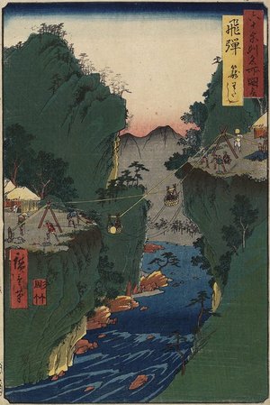
Many posts about GANs online use the MNIST dataset or the CelebA faces dataset; for this series, I’ll using more challenging datasets to better represent the difficulties of training these algorithms in the wild. As in my earlier post, all the experiments below use images from the Japanese Woodblock Print database.

Let’s try and generate images like the one above!

I’ll skip the steps of defining the dataset and dataloader since they’re usually pretty simple and instead focus on the training loop. If you’d like to see that code, you can check out the full repo here.

First, let’s initialize both our models and optimizers. We’re using a learning rate of 2e-4 as per the DCGAN paper.

        
d_net  =  Discriminator()
d_net.to(device)
d_optimizer  =  optim.Adam(d_net.parameters(), lr=2e-4, betas=(0.5, 0.999))

g_net  =  Generator()
g_net.to(device)
g_optimizer  =  optim.Adam(g_net.parameters(), lr=2e-4, betas=(0.5, 0.999))
    

Same as last time, I find it helpful to define a fixed latent batch at the beginning of training, to use as a comparison throughout training to see how the GAN improves generating for the same latents $z$ . I’ll also add in an array to track loss statistics throughout training, and values to define our real and fake labels for our loss computations.

        
fixed_latent  =  torch.randn(64, 128, 1, 1, device=device)

d_losses_real  = []
d_losses_fake  = []
g_losses  = []

real_label  =  1.
fake_label  =  0.
    

Now we can define our actual training loop. One consideration that we have to deal with is that in practice, we can’t actually simultaneously update $G$ and $D$ - that’s just not how computers work. We have to define an iterative approach to this game that slowly updates both $G$ and $D$ . In the original paper, the authors defined a hyperparameter $k$ that signified how many times $D$ would be updated each epoch before $G$ is updated, although in practice this is often set to $k=1$ .

In our implementation, we’ll iterate through our dataloader in batches for each epoch during training, performing one gradient update on $D$ and then $G$ . Let’s start with the easy stuff -

        
for  epoch  in  range(n):
    for  i, batch  in  enumerate(dataloader, 0):
        batch, _  =  batch
        batch  =  batch.to(self.args.device)
        batchsize  =  batch.shape[0]
    

The rest of the code will go within the second for loop. First, we have to generate a batch of fake inputs i.e. $G(z)$ .

        
noise  =  torch.randn(batchsize, 128, 1, 1, device=device)
fake_batch  =  g_net(noise)
    

We can generate our labels now that we know how big the batch is.

        
real_labels  =  torch.full((batchsize,), real_label, dtype=torch.float, device=device)
fake_labels  =  torch.full((batchsize,), fake_label, dtype=torch.float, device=device)
    

Recall that for the discriminator, we want to maximize the following expression
$$\mathbb{E}_{x\sim p_{data}(x)} [\log D(x)] + \mathbb{E}_{z\sim p(z)} [ \log (1 - D(G(z)))]$$
We’re going to split the discriminator update into two parts. First, we’re going to compute the gradients for the discriminator on the real inputs i.e. $\mathbb{E}_{x\sim p_{data}(x)} [\log D(x)]$ .

Let’s recall the expression for binary cross entropy loss: $-\left[ y \log x + (1 - y) \log (1 - x) \right]$ . What happens when we set $y = 1$ ? We get $-\log x$ , which is pretty much exactly what we want. If we minimize this quantity, it’ll be the same as maximizing $\log x$ .

This presents a pretty easy way to maximize $\mathbb{E}_{x\sim p_{data}(x)} [\log D(x)]$ - we just minimize the binary cross entropy loss between $D(x)$ and $\mathbf{1}$ , which is our vector real_labels:

        
import torch.nn.functional as F
...

d_net.zero_grad()

output  =  d_net(batch).view(-1)
d_loss_real  = F.binary_cross_entropy(output, real_labels)
d_loss_real.backward()

# D(x)
dx  =  output.mean().item()
    

We can do a similar trick for the other term we need to maximize - $\mathbb{E}_{z\sim p(z)} [ \log (1 - D(G(z)))]$ . Again, let’s recall the binary cross entropy loss $-\left[ y \log x + (1 - y) \log (1 - x) \right]$ . If we set $y = 0$ here, we get $-\log (1 - x)$ , which is exactly what we want. If we minimize this quantity, it’ll be the same as maximizing $\log (1 - x)$ .

The implementation is pretty simple - we minimize the binary cross entropy loss between $D(G(z))$ and $\mathbf{0}$ , which is our vector fake_labels:

        
output  =  d_net(fake_batch.detach()).view(-1)
d_loss_fake  =  bce(output, fake_labels)
d_loss_fake.backward()

# D(G(z))
dgz_1  =  output.mean().item()

d_optimizer.step()
    

You may notice that we only call the optimizer after the second backward call. This is on purpose - PyTorch will automatically accumulate the gradients from multiple backward calls for us, so we don’t have to add the losses and propagate them together. Another important thing here is that we .detach() the fake batch here because we don’t want to have the gradients from $G$ when we’re optimizing for $D$ .

Now we can write the code for the generator update. Recall that for the generator, we want to minimize $\mathbb{E}_{z\sim p(z)} [ \log (1 - D(G(z)))]$ . One tip that the authors of the original paper recommended for this part is maximizing $\log D(G(z))$ instead of minimizing $\log (1 - D(G(z)))$ , for better gradient flow in the early iterations of training.

Maximizing $\log D(G(z))$ is the same as minimizing $-\log D(G(z))$ , which means we can use the binary cross entropy loss again, with $y = 1$ and the generated output prediction $D(G(z))$ . Importantly, we don’t .detach() the fake batch here because we want to have the gradients from $G$ flow backward.

        
g_net.zero_grad()

output  =  d_net(fake_batch).view(-1)
g_loss  =  bce(output, real_labels)
g_loss.backward()

# D(G(z))
dgz_2  =  output.mean().item()
    
g_optimizer.step()
    

As in my earlier post, I usually like to track the progress of training at fixed intervals by generating a batch using a fixed latent. You can compare this batch throughout training to get a sense of how the GAN improves.

        
if (i  %  1000  ==  0):
    g_net.eval()
    fake  =  g_net(fixed_latent).detach()
    g_net.train()
    

And we’re ready to train!

In my experiments, I ran the training for 25 epochs, using a learning rate of 2e-4, a batch size of 128, and a latent size of 128. Let’s see how it did. For each image below, I’ve put a generated image from our GAN as well as an image from the dataset that I thought looked similar.

Let’s also take a look at how the GAN improved on the same batch of latent inputs ( fixed_latent) from above throughout training.

As you can see, the GAN pretty quickly improves from just random noise into some decent images. Later on, the features in each image improve as well as the overall image diversity, creating some pretty stunning results, even if they’re not quite recognizable as art.

For completeness, let’s also visualize a few interpolations of the generated images over the latent space $z$ , like we did for the VAE article. We’ll generate two random vectors, and interpolate between those vectors, generating images for each. The code for interpolating between two points is pretty standard but I’ve also included some plotting code below in case its useful.

		
def  interpolate_points(p1, p2, n_steps=8):
	ratios  =  np.linspace(0, 1, num=n_steps)
	vectors  = []
	for  ratio  in  ratios:
		v  = (1.0  -  ratio) *  p1  +  ratio  *  p2
		vectors.append(v)
	return  vectors

def  plot_generated(examples):
	for  i  in  range(len(examples)):
		plt.subplot(1, len(examples), 1  +  i)
		plt.axis('off')
		plt.imshow(examples[i])
	plt.subplots_adjust(wspace=0, hspace=0)
	plt.savefig("interp.png", bbox_inches='tight')

# pick two random points to interpolate between
z0  =  torch.randn((512, 1, 1))
z1  =  torch.randn((512, 1, 1))

# get the interpolated points
zs  =  interpolate_points(z0, z1)
zs = [z0] + zs + [z1]

# run the points through the generator
image_interps  = [g_net(z).squeeze() for  z  in  zs]
image_interps  = [image.permute(1, 2, 0).detach().numpy() for  image  in  image_interps]

# plot the generated images
plot_generated(image_interps)
	

And we have our results below:

Overall, we're able to get some pretty good results. Our GAN definitely improved on the VAE from last time but still struggles with the really fine details in each image. The GAN also seems like it isn't fully encapsulating the features in each image of the original dataset, which shows in the final generations.

Common Problems

---

We were able to achieve pretty good results from our GAN, but in general training one can be difficult. GANs are notorious for being extremely sensitive to hyperparameters during training. Earlier, we showed the existence of the global minimum for this algorithm, as well as given some bounds on what the theoretical optimums are. However, there are some other considerations we can analyze that relate to the main problems you’re likely to run into when training GANs:

1. Non-convergence.

   This is the most standard problem that plagues GANs - when the generator and discriminator don’t reach an equilibrium in the minimax game. We proved that there was a unique solution above, but we never showed that it was possible to always reach it. For a sufficiently complex problem, its possible that a GAN could never converge. In those scenarios, it is usually useful to slow the learning rate, acquire more data, increase the latent size input to the generator, or in general play around with the hyper-parameters of the model.

2. Mode collapse.

   We could also consider the scenario where the generator $G$ improves faster than the discriminator $D$ . In this scenario, it is possible that the generator will tend to produce images that look very similar to each other - in math terms, the generator maps multiple inputs $z$ to the same output $x$ , resulting in very similar outputs in the data space.

   This often occurs when the generator $G$ reaches a stable state faster than the discriminator $D$ . When that happens, $G$ will often try and generate one optimal output $x^*$ that fools $D$ the most. In doing so, every single output from $G$ will resemble or be the same as $x^*$ . This is a pretty simplified explanation, as the true reasons behind mode collapse are still under research, but a common solution that sometimes works in practice is to update the discriminator more frequently (i.e. changing the value of $k$ from $1$ to something else).

3. Diminished gradient.

   Consider the scenario that occurs when $D$ reaches a high accuracy, while $G$ is still not quite good yet. In math terms, $D(x)$ is close to $1$ when $x \sim p_{data}(x)$ , while $D(x)$ is close to $0$ when $x \sim p_{g}(x)$ . In this case, the term for the generator $G$ in the minimax game, i.e. $\mathbb{E}_{z\sim p(z)} [ \log (1 - D(G(z)))]$ becomes $\mathbb{E}_{z\sim p(z)} [\log 1] = 0$ . Similarly, the term for $D$ , $\mathbb{E}_{x\sim p_{data}(x)} [\log D(x)]$ , also becomes $\mathbb{E}_{x\sim p_{data}(x)} [1] = 0$ . As you can see, if this scenario were to happen, there is no gradient from which the generator $G$ can learn how to properly fool the discriminator $G$ . Qualitatively, when training a GAN, you don’t want the discriminator $D$ to get too good too early, because it becomes impossible for the generator $G$ to fool it.

   One solution that the authors of the original paper proposed for this issue is to replace the objective for $G$ . Recall that for $G$ , we want to minimize $\mathbb{E}_{z\sim p(z)} [ \log (1 - D(G(z)))]$ . I’ll skip the derivation here, but maximizing $\mathbb{E}_{z\sim p(z)} [ \log D(G(z))]$ is basically equivalent to the above, and it avoids some of the issues where $\log (1 - D(G(z)))$ can approach $0$ early in training. In practice, it’s pretty common to use this as the objective for $G$ instead of the original formulation.

Tips and Tricks

---

Fortunately, there are some small, easy to implement tricks we can add to our implementation that can stabilize training and significantly improve the overall results. The first two techniques below are from this 2016 paper from OpenAI.

1. One-sided label smoothing

   The idea behind label smoothing is that using smoothed values like $0.9$ instead of $1$ for the binary cross entropy objective can make the objective function a little nicer. In mathematical terms, we replace the optimal discriminator with
   $$D^*(x) = \frac{\alpha p_{data}(x)}{p_{data}(x) + p_{g}(x)}$$ where $\alpha = 0.9$ . In our code, this only requires changing it to real_label = 0.9. The OpenAI paper also provides some reasoning for why smoothing the fake_label is undesirable, resulting in a one-sided label smoothing.

2. Feature matching objective

   Feature matching is a proposed change to the generator objective. Essentially, instead of directly maximizing the output of the discriminator, the generator is instead trained to match the features that the discriminator uses in an intermediate layer. The idea is that the generator should learn to value and emulate the same things that the discriminator is using to make its evaluation.

   In PyTorch, this requires some pretty significant changes so I won’t show it all here. Essentially, to implement this feature you’d have to add a forward hook that returns the output of some intermediate layer of the discriminator network. Then, instead of the binary cross entropy objective for the generator, you’d compute the mean squared error between the features of the discriminator from a real batch forward pass and the features from a fake batch forward pass.

3. Conditional labeling

   If you have labels for your dataset, one small addition that could help your GAN is to include your labels as part of the input to your GAN. This is called conditioning the input on some other information (in this case, the label). Doing this gives your GAN more semantic information about each of the classes of images in your dataset, and allows it to be more representative overall.

   To make this change, you would have to include an embedding layer in the generator $G$ , as well as change the output of the discriminator to a vector based on the number of classes you have. Of course, this would mean you would have to replace binary cross entropy with regular cross entropy, in addition to changing the way your labels work for that objective.

   TLDR, if you have labels in your dataset, definitely try and use them.

4. Spectral normalization

   Spectral normalization is an approach designed to combat the exploding gradient and vanishing gradient problem that sometimes occurs when training GANs. This can result in instability in the training procedure and can be quite difficult to fix.

   Spectral normalization requires some prerequisites. If you use activation functions that are 1-Lipschitz continuous (which basically just means that the maximum absolute value of the derivative for the function is 1), such as LeakyReLU, and you ensure the spectral norm of the weights is $1$ , the norm of the gradients will be limited by the size of the network. There’s a lot more theory behind this in the paper if you’re interested, but for our purposes all that we need to do is wrap every Conv2d call in the discriminator $D$ with the spectral norm function, like below

               
   import  torch.nn.utils.parametrizations  as  P
   ...
   P.spectral_norm(nn.Conv2d(input, output, kernel, 2, 1, bias=False))
           

   This is a pretty easy addition to make that can help massively later on with training stability.

If you’d like even more tricks for your GAN experiments, check out the ganhacks repo - I found this really helpful when I was first starting out with my own tests. Even with all the tricks above, it’s very likely that you’ll require some additional fine-tuning for your dataset.

GANs are notoriously difficult to train and require a lot of experimentation to achieve really good results. They’re a bit more difficult to use in production because of this, which is why algorithms like diffusion are preferred for state of the art image generation algorithms like Stable Diffusion. Diffusion models are also known for their incredible detail, which we can hopefully achieve some examples of in the next part of this series.

If you’d like to check out the full code for this series, you can visit my public repository.

---