Machine Learning Fundamentals: Linear Classification (2/2)
Introduction
In my previous article, I covered the basics of the classification problem and some techniques we’ll need for the future. Now, we’ll dive deeper into linear classification, building off of the topics covered last time.
As from before, my goal with this series is to serve as an educational tool for those looking to review the fundamentals of machine learning with an emphasis on ease of understanding. This series assumes some familiarity with machine learning in general, and as such I will try to focus on the underlying mathematics and intuition behind the concepts that we discuss.
Linear Classification
Last time, we discussed the general problem of classification, and built up from the Bayes classifier into something practical - namely, using MLE estimates, we derived a class-conditional classifier where we assume each class can be modeled by a Gaussian distribution.
One thing you may realize now is that for classification, we don’t strictly need the actual parameters of the distribution for each class. It’s useful in some cases, but if we’re considering solely our ability to tell whether something is one class or the other, we don’t really use the parameters themselves. Rather, we use the boundary between classes to discern whether a sample is one or the other (you can see these boundaries above).
Let’s focus on these decision boundaries. Mathematically, for two classes \(a\) and \(b\) and class-conditional classifiers \(f_a(x)\) and \(f_b(x)\) we can write the decision boundary between them as the set of points where \(f_a(x) = f_b(x)\) or equivalently when \(f_a(x) - f_b(x) = 0\). Here’s where we get to the linear part (finally) - for many use cases, it’s much simpler to model the decision boundary directly, and this can just be a line!
Linear Discriminant Analysis
Let’s return to a familiar example from last article - namely, we model each class conditional distribution \(p_k(x)\) as a multivariate Gaussian parameterized by \(\mu_k, \Sigma_k\) as follows \[p_{k}(x) = \frac{1}{\sqrt{(2\pi)^d|\Sigma_k|}}\exp\left(-\frac{1}{2}(x-\mu_k)^T\Sigma_k^{-1}(x-\mu_k)\right)\] Instead of the actual probabilities, let’s focus on the decision boundary between two classes \(a\) and \(b\). If we let \(\pi_k\) be the associated prior for the class \(k\), we can analyze the quantity \(f_k(x) = p_k(x)\pi_k\).
We’ll use the log trick I mentioned last time to analyze this quantity easily. Instead of directly analyzing \(f_k(x)\), we’ll analyze
\(\log f_k(x)\), since for this analysis we don’t care about the absolute magnitude of this function. We have
\[\begin{align*}
\log f_k(x) &= \log p_k(x) + \log \pi_k\\
&= \log \left[ \frac{1}{\sqrt{(2\pi)^d|\Sigma_k|}}\exp\left(-\frac{1}{2}(x-\mu_k)^T\Sigma_k^{-1}(x-\mu_k)\right) \right] + \log \pi_k\\
&= \log \left[ (2\pi)^{-\frac{d}{2}}|\Sigma_k|^{-\frac{1}{2}} \right] - \frac{1}{2}(x-\mu_k)^T\Sigma_k^{-1}(x-\mu_k) + \log \pi_k \\
&= -\frac{d}{2} \log 2\pi -\frac{1}{2} |\Sigma_k|- \frac{1}{2}(x-\mu_k)^T\Sigma_k^{-1}(x-\mu_k) + \log \pi_k \\
\end{align*}\]
Since the first term is a constant, it is the same for all values of \(k\), meaning that if we wanted to analyze the quantity \(f_a(x) - f_b(x)\),
we can just drop this value. We can now define the quadratic discriminant analysis (QDA) function \(\delta_k(x)\)
as follows
\[\delta_k(x) = -\frac{1}{2}
\log |\Sigma_k|- \frac{1}{2}(x-\mu_k)^T\Sigma_k^{-1}(x-\mu_k) + \log \pi_k\]
This function is quadratic because of the middle term (we have two factors of \((x - \mu_k)\). We also call this function
discriminatory because we can define the decision boundary between two classes \(a\) and \(b\) by the set \(\{x: \delta_a(x) = \delta_b(x)\}\)
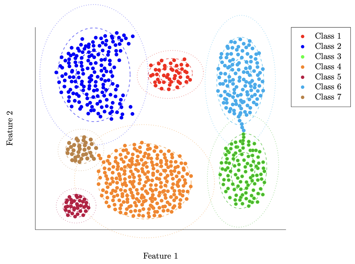
i.e. these functions allow us to discriminate between two classes \(a\) and \(b\). For the sake of visualization, let’s plot these boundaries
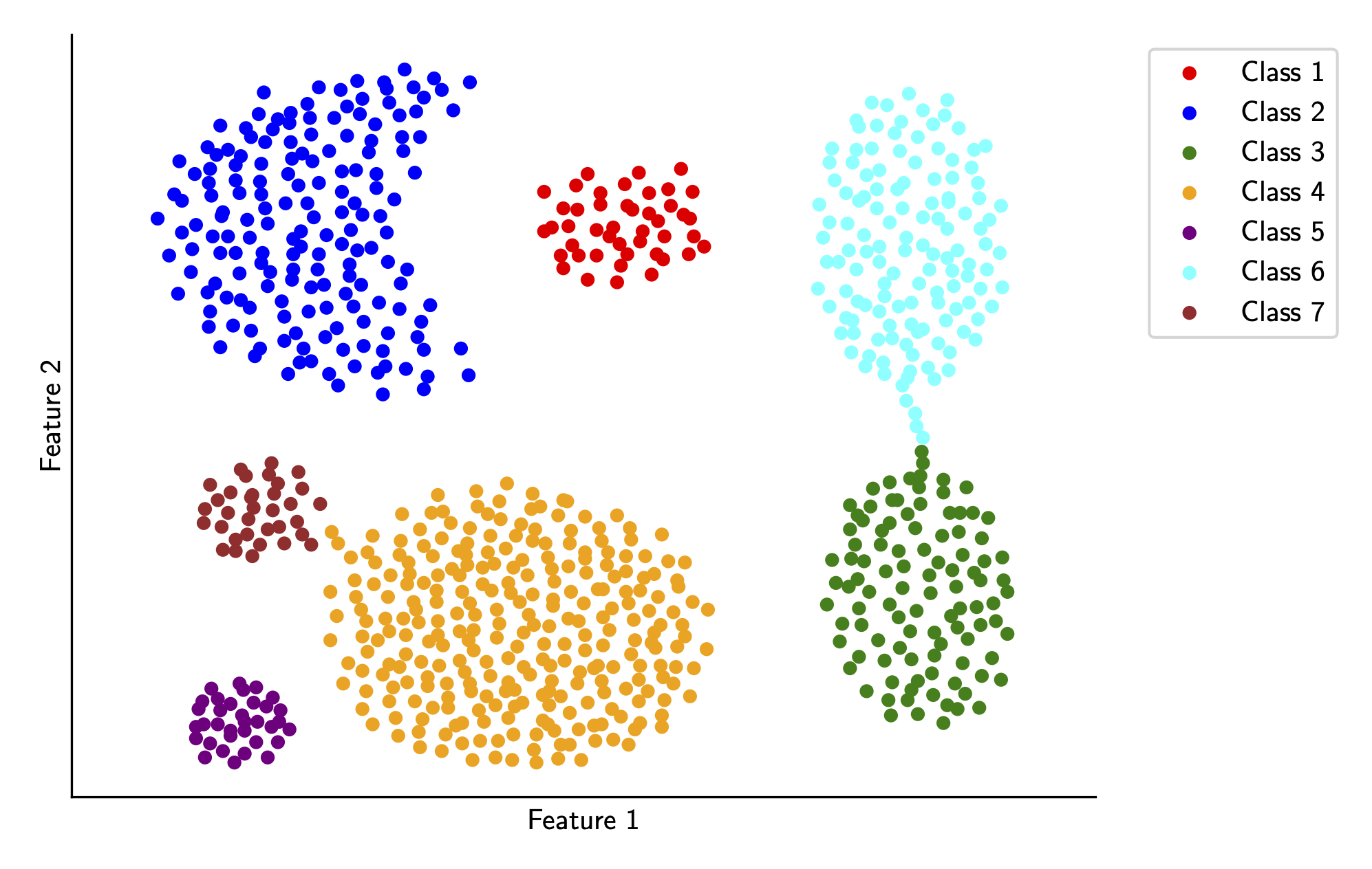
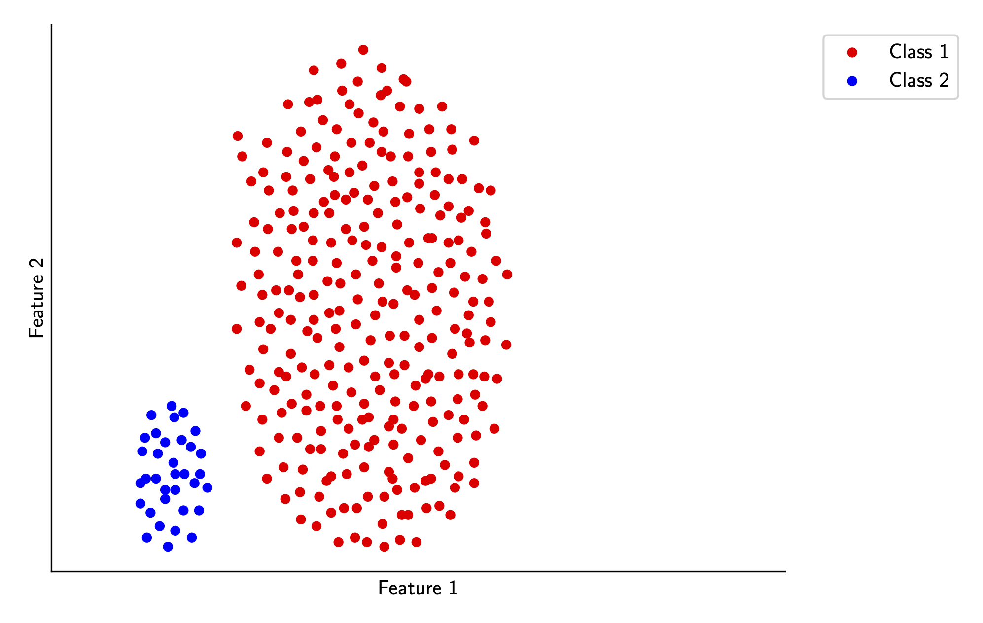
on our sample data from last article. As a reminder, here’s that again
To compute the coefficients of the QDA function for each class, we simply use our MLE estimates from last time. In code, this is pretty simple
qda_coefficients = {}
for c in CLASSES:
    sigma_inv = np.linalg.inv(mle_fits[c]['sigma'])
    log_det_sigma = np.log(np.linalg.det(mle_fits[c['sigma']))
    mu = mle_fits[c]['mu']
    prior = mle_fits[c]['prior']

    # put in form x^TAx + bx + c for vector valued x
    # Quadratic coefficient matrix
    A = -0.5 * sigma_inv

    # Linear coefficient vector
    b = sigma_inv @ mu

    # Constant term
    constant = -0.5 * (mu.T @ sigma_inv @ mu) - 0.5 * log_det_sigma + np.log(prior)

    qda_coefficients[int(c)] = {
        'A': A, # 2x2 quadratic coefficient matrix
        'b': b, # 2x1 linear coefficient vector
        'c': constant, # scalar constant term
    }
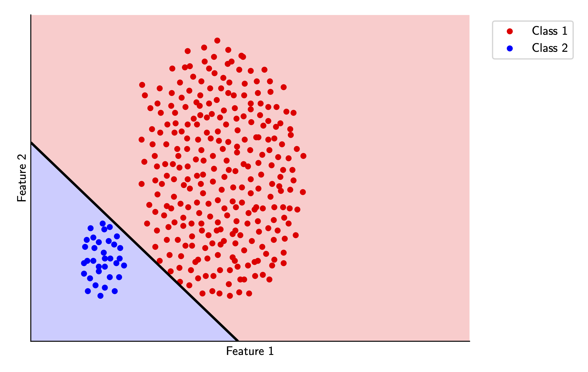
We can use these QDA functions to compute decision boundaries for every pair of classes and then plot these. If you’d like to see all the code for this article, take a look here. Plotting these decision boundaries results in the following
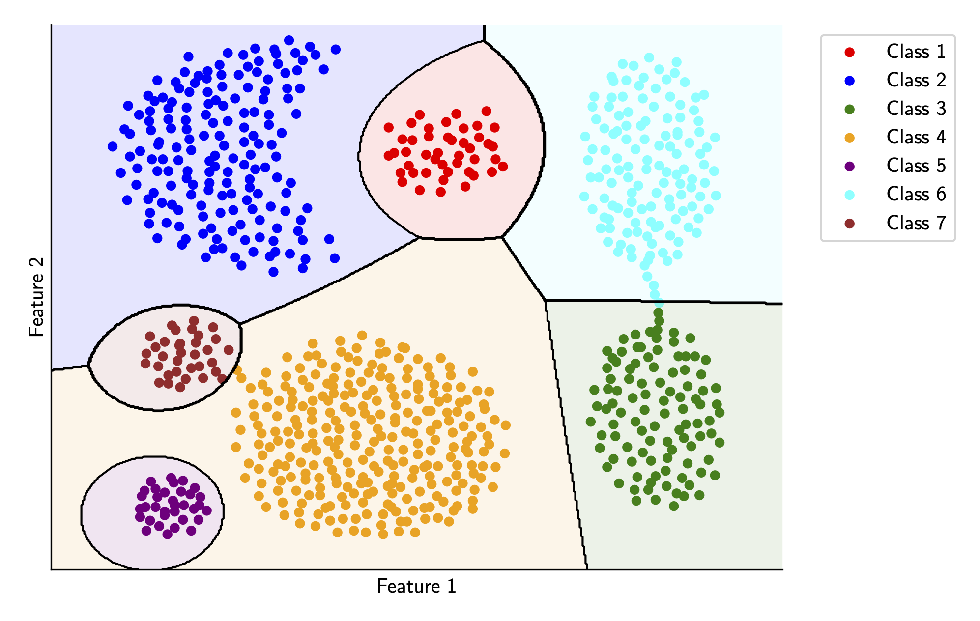
Pretty solid! Although we do have some weird things going on for Class 1, Class 5, and Class 7. Ideally, we’d like our decision boundaries to be as simple as possible, which motivates our next step.
Let’s take a look at the QDA function definition again \[\delta_k(x) = -\frac{1}{2} \log |\Sigma_k|- \frac{1}{2}(x-\mu_k)^T\Sigma_k^{-1}(x-\mu_k) + \log \pi_k\] This is good, but remember that in the end, what we’re actually looking at to determine the decision boundary between two classes \(a\) and \(b\) is \(\delta_a(x) - \delta_b(x)\). Why don’t we look at that quantity directly? \[\begin{align*} \delta_a(x) - \delta_b(x) = &-\frac{1}{2} \log |\Sigma_a|- \frac{1}{2}(x-\mu_a)^T\Sigma_a^{-1}(x-\mu_a) + \log \pi_a\\ &+ \frac{1}{2} \log |\Sigma_b| + \frac{1}{2}(x-\mu_b)^T\Sigma_b^{-1}(x-\mu_b) - \log \pi_b\\ = &-\frac{1}{2}(x-\mu_a)^T\Sigma_a^{-1}(x-\mu_a) + \frac{1}{2}(x-\mu_b)^T\Sigma_b^{-1}(x-\mu_b) \\ &+ -\frac{1}{2}(\log |\Sigma_a| - \log |\Sigma_b|) + \log \pi_a - \log \pi_b\\ = & -\frac{1}{2} \left( \left[x^T\Sigma_a^{-1}x - x^T\Sigma_b^{-1}x\right] - 2\left[\mu_a^T\Sigma_a^{-1} - \mu_b^T\Sigma_b^{-1} \right]x+ \mu_a^T\Sigma_a^{-1}\mu_a - \mu_b^T\Sigma_b^{-1}\mu_b \right) \\ &-\frac{1}{2}(\log |\Sigma_a| - \log |\Sigma_b|) + \log \pi_a - \log \pi_b\\ \end{align*}\] Here, we’re kind of stuck. However, one thing we can notice is that the only quadratic term of \(x\) in this equation is \(x^T\Sigma_a^{-1}x - x^T\Sigma_b^{-1}x\). If it happened to be the case that \(\Sigma_a = \Sigma_b\), then we could remove the quadratic dependency all together and end up with a linear decision boundary!
This is the key assumption behind linear discriminant analysis (LDA). We assume that all class covariances are actually equivalent i.e. instead of
\(\Sigma_k\), we assume one global covariance \(\Sigma\). Let’s continue our simplification of \(\delta_a(x) - \delta_b(x)\)
with this in mind.
\[\begin{align*}
\delta_a(x) - \delta_b(x) = &-\frac{1}{2} \left( \left[x^T\Sigma^{-1}x - x^T\Sigma^{-1}x\right] - 2\left[\mu_a^T\Sigma^{-1} - \mu_b^T\Sigma^{-1} \right]x+ \mu_a^T\Sigma^{-1}\mu_a - \mu_b^T\Sigma^{-1}\mu_b \right) \\ &-\frac{1}{2}(\log |\Sigma| - \log |\Sigma|) + \log \pi_a - \log \pi_b\\
= &-\frac{1}{2} \left[-2(\mu_a^T - \mu_b^T)\Sigma^{-1} x+ \mu_a^T\Sigma^{-1}\mu_a - \mu_b^T\Sigma^{-1}\mu_b \right] + \log \pi_a - \log \pi_b\\
=& (\mu_a - \mu_b)^T\Sigma^{-1}x -\frac{1}{2}(\mu_a^T\Sigma^{-1}\mu_a - \mu_b^T\Sigma^{-1}\mu_b) + \log \pi_a - \log \pi_b\\
\end{align*}\]
This is a linear equation! If you think of each term as follows
\[
\underbrace{(\mu_a - \mu_b)^T \Sigma^{-1} \vphantom{-\frac{1}{2} (\mu_a^T \Sigma^{-1} \mu_a - \mu_b^T \Sigma^{-1} \mu_b) + \log \pi_a - \log \pi_b}}_{w^T} x
+
\underbrace{-\frac{1}{2} (\mu_a^T \Sigma^{-1} \mu_a - \mu_b^T \Sigma^{-1} \mu_b) + \log \pi_a - \log \pi_b}_{b}
\]
you can then write \(\delta_a(x) - \delta_b(x) = w^Tx + b\), a linear decision boundary. The linear discriminant function for each class \(k\)
then can be written (overloading the notation we used for QDA earlier) as
\[\delta_k(x) = \mu_k^T\Sigma^{-1}x -\frac{1}{2}\mu_k^T\Sigma^{-1}\mu_k + \log \pi_k\]
Now let’s revisit our assumption of a common class covariance \(\Sigma\). We need to fit this covariance to all our input data, using MLE (covered last time). The derivation ends up being very similar, so I won’t cover it explicitly, but in the end the MLE estimate of \(\Sigma\) for LDA ends up being \[\Sigma_{LDA} = \frac{1}{N}\sum_{c=1}^C n_c \hat{\Sigma}_c\] where \(N\) is the total number of training samples, \(n_c\) is the number of samples in the class \(c\), and \(\hat{\Sigma}_c\) is our MLE estimate of the class conditional covariance. Essentially, we’re weighting each class covariance by the number of samples and averaging over all samples for the global covariance.
Let’s see how this works on our sample dataset! The code is very similar in style to the QDA code above, but much simpler to implement since we don’t have any of those nasty quadratic terms to handle.
lda_coefficients = {}

# estimate global covariance
sigma_lda = np.zeros_like(mle_fits[1]['sigma'])
for c in CLASSES:
	n_c = len(df[df['class'] == c])
	sigma_lda += n_c * mle_fits[c]['sigma']
	sigma_lda /= len(df)  # 1/N
	sigma_lda_inv = np.linalg.inv(sigma_lda)

for c in CLASSES:
	mu = mle_fits[c]['mu']
	prior = mle_fits[c]['prior']

	# put in form wx + b for vector valued x
	# Linear coefficient vector
	w = sigma_lda_inv @ mu

	# Constant term
	b = -0.5 * (mu.T @ sigma_lda_inv @ mu) + np.log(prior)
	lda_coefficients[int(c)] = {
		'w': w,  # 2x1 linear coefficient vector
		'b': b,  # scalar constant term
	}
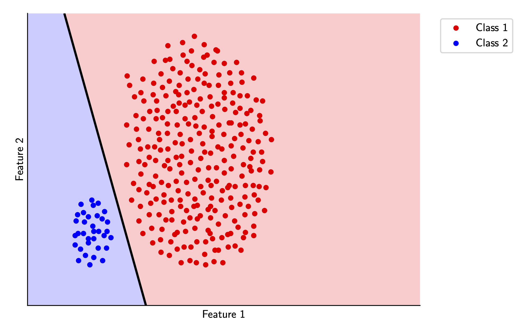
Our code to determine the decision boundaries is even easier than before - we can just subtract the coefficients for the relevant discriminant functions and end up with the linear decision boundary between the two classes. Again, if you’d like to see the code, its all available here. Let’s visualize what our decision boundaries look like.
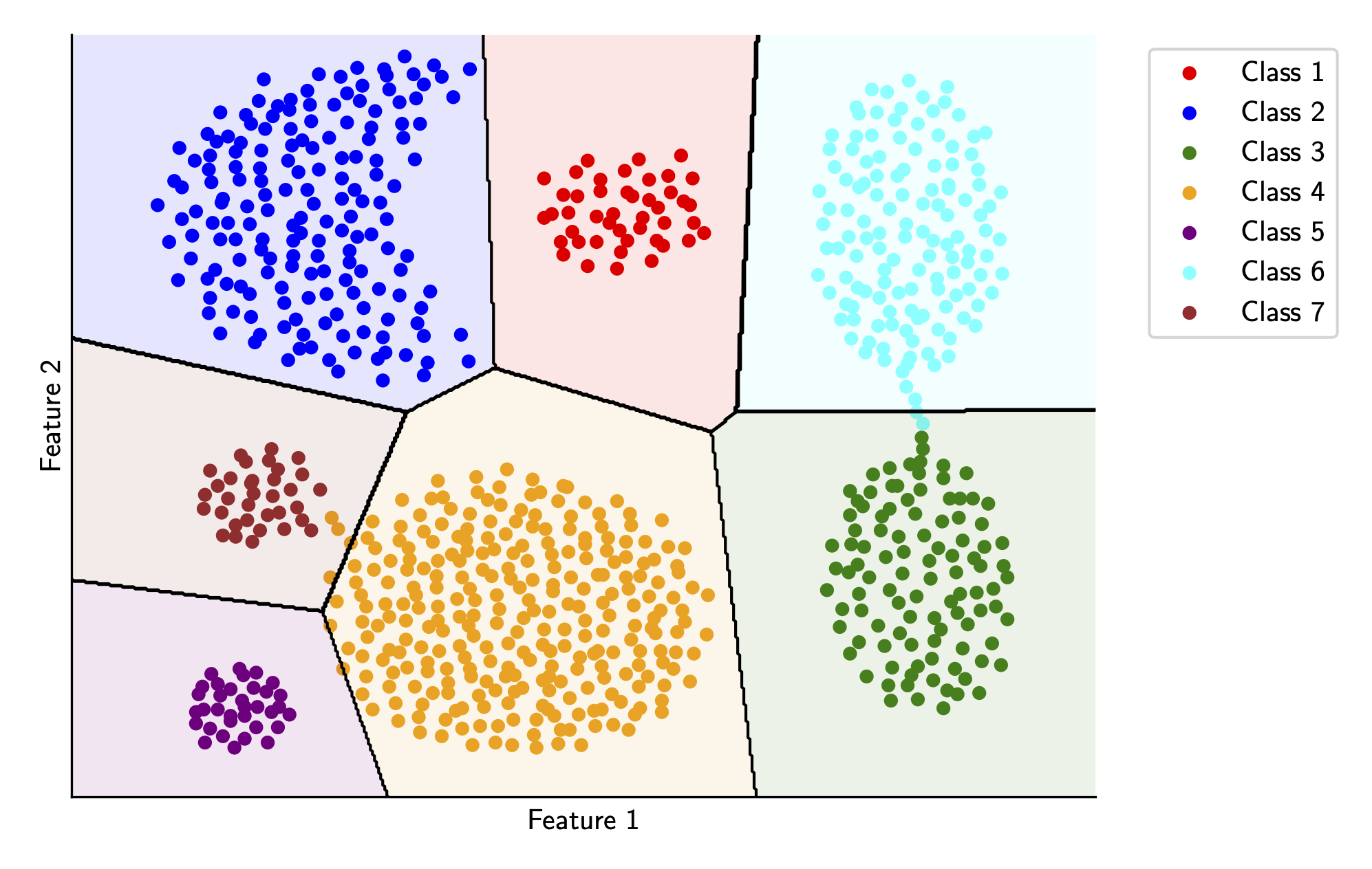
These boundaries aren’t as accurate as the QDA boundaries, which is to be expected since we’re making a big assumption about the global covariance matrix, but they’re still surprisingly good! Furthermore, these boundaries are likely to be more generalizable since they don’t fit super heavily on the training data.
Perceptron Algorithm
You may notice from our work on linear discriminant analysis above that our linear decision boundaries aren’t exactly optimal. We could definitely visualize more accurate decision boundaries, especially for the cases when the two classes appear to be linearly separable i.e. there is a linear decision boundary that can perfectly separate the data.
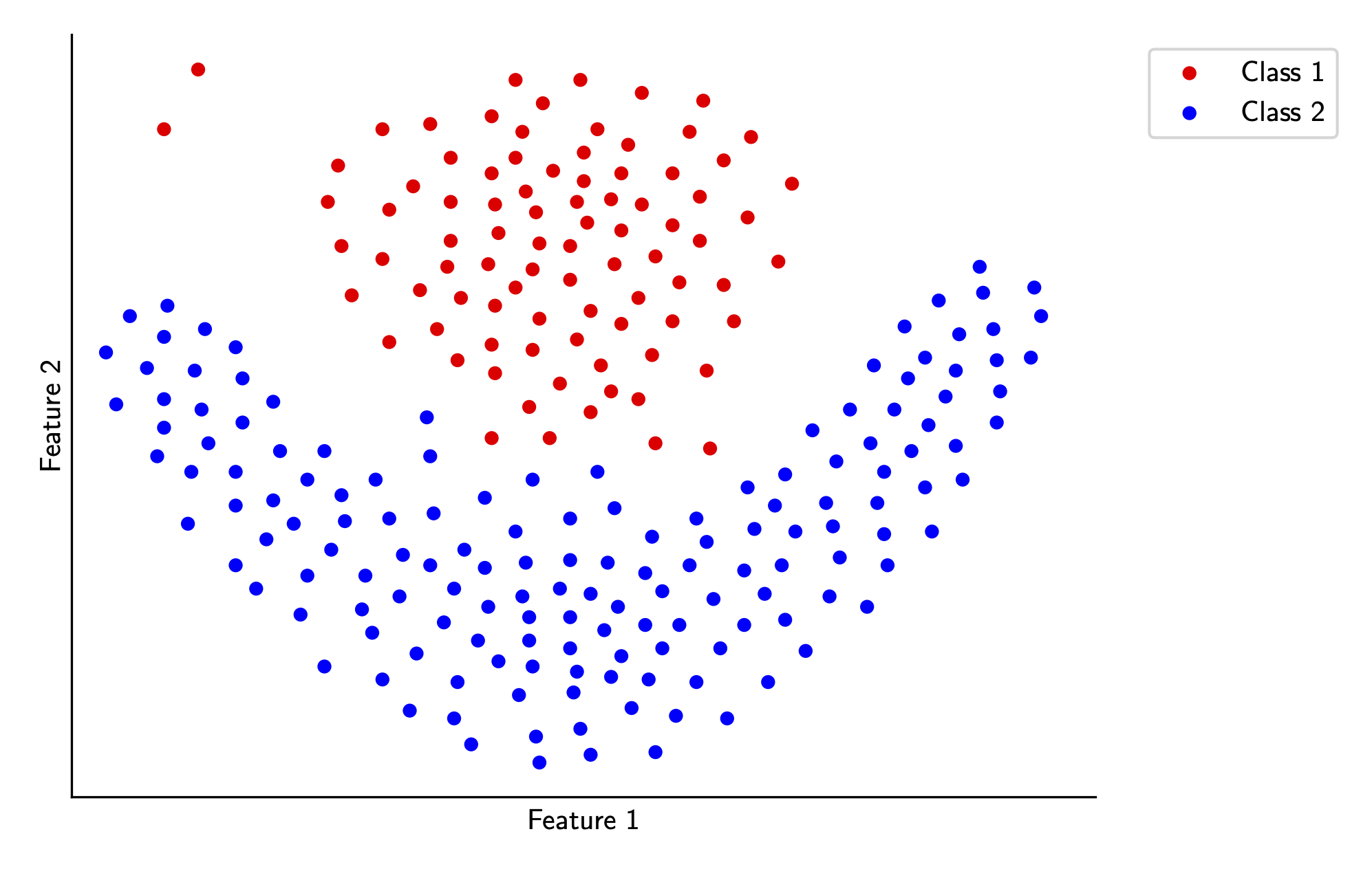
For this section, we’ll look at a simplified problem. We’ll limit our analysis to two linearly separable classes from our original sample data, as shown below. To extend this (and the following algorithms) to the non-binary case, we can just train \(k\) separate classifiers for each class, where one class is treated as the positive class and all other classes are treated as the negative class.
Mathematically, we assume training data \(X, Y\), where \(y_i \in \{-1, 1\}\). We want to find a vector \(w\) and a bias term \(b\) such that \(w \cdot x_i \geq 0\) if \(y_i = 1\) and \(w \cdot x_i \leq 0\) if \(y_i = -1\), which will classify each sample correctly. Equivalently, we can write this as \[ y_i(w \cdot x_i + b) \geq 0 \] for all input pairs \((x_i, y_i)\).
First, let’s simplify our equation a little bit. Let’s express our equation fully in terms of vectors - we can write \[ \begin{align*} y_i(w \cdot x_i + b) &\geq 0\\\\ y_i \left( \begin{bmatrix} w\\ b \end{bmatrix} \cdot \begin{bmatrix} x_i\\ 1 \end{bmatrix} \right)&\geq 0 \end{align*} \] Notice that if we include this extra \(1\) in our vector for \(x_i\) , we can just represent the entire equation with one weight vector instead of requiring both a weight vector and a bias term. So let’s just add this extra dimension to all our samples in \(X\)! This trick is called lifting because we’re essentially taking the \(d\)-dimensional data we have currently and transforming it into a \(d+1\) dimensional dataset i.e. we’re raising (or lifting) the dimension of our input data.
Under this new assumption, our original objective becomes to find a weight vector \(w\) (with \(d+1\) dimensions) that satisfies \[ y_i (w \cdot x_i) \geq 0 \] for all input pairs \((x_i, y_i)\), and with the bias term included in each \(x_i\).
Let’s quantify how “wrong” a choice of \(w\) can be in this setting. There’s two cases - either we get it right or wrong. Mathematically, our predicted classification will be
\(\text{sign}(w \cdot x_i)\). Our training error or cost across the entire dataset is just the fraction we are incorrect, which mathematically can be written as follows
\[
C(w) = \frac{1}{n} \sum_{i}^n \mathbf{1}[\text{sign}(w \cdot x_i) \neq y_i]
\]
which we want to minimize over \(w\).
Here we run into a problem. We can’t use the standard technique with this function of taking the derivative and analyzing the stationary points because of the \(\text{sign}\) and indicator functions, which don’t have defined derivatives everywhere.
However, we’re not completely stuck - if we do classify a point correctly, the indicator function in the above cost function contributes \(0\) to the end training error. In essence, our training error only depends on the misclassified points! Therefore, instead of looking at all the samples points, let’s write our cost function only in terms of points that we are currently misclassifying.
When we misclassify a point, that means that \(y_i(w \cdot x_i) \leq 0\). Therefore, we can write \[ C(w) = \frac{1}{n} \sum_{i \in W} -y_i (w \cdot x_i) \] where the set \(W\) is the set of all misclassified points.
This function has a clear gradient with respect to \(w\), which means we can use our tricks from earlier - but there’s a catch. Since we’re limiting our cost function to the set \(W\), we aren’t guaranteed global optimality. Furthermore, every time we update \(w\), we might misclassify old points that were correctly classified earlier.
But here’s where our assumption from earlier comes into play - since we know that there exists some \(w\) that does classify all points correctly we know that there is a global minimum for the original cost function. Therefore, we can use gradient descent with our new objective function to find a \(w\) that satisfies our original constraints. I won’t directly cover gradient descent in this article (perhaps in a future article), but for a brief overview I found this resource very helpful.
This is the basis for the perceptron algorithm, defined as such (using stochastic gradient descent with learning rate \(\alpha\)).
For \(t=1, 2, \dots\) if there exists \((x_i, y_i)\) s.t. \(\text{sign}(w_t \cdot x_i) \neq y_i\),
update \(w_{t+1} = w_t + \alpha y_i x_i\), otherwise return \(w_t\)
Intuitively, we just keep updating \(w\) with the gradient with respect to all the misclassified points until no misclassified points remain. You might be skeptical of this - after all, how can we guarantee this algorithm actually terminates?
Let’s prove it. We’ll call the optimal weight vector \(w^*\), which classifies every point correctly. We’ll further assume that \(w^*\) has unit length and can separate the training samples with a margin of \(\gamma\) i.e. \(y_i (w^* \cdot x_i) \geq \gamma\) for arbitrary \(x_i, y_i\).
At iteration \(t\), let’s analyze how far \(w_t\) can be from \(w^*\). Due to our earlier trick of adding the bias vector, we know that the hyperplane separating our points goes through the origin, meaning that the normal vector for that hyperplane also starts from the origin. Geometrically, we’re just rotating \(w_t\) until it aligns with \(w^*\), which motivates the choice of cosine distance for our distance metric. Recall the cosine distance between two vectors \(a, b\) \[ \cos(\theta) = \frac{a \cdot b}{\lVert a \rVert \, \lVert b \rVert} \] For our scenario, let’s look at the numerator and denominator separately.
First, \(w_t \cdot w^*\). Using the update rule from the perceptron algorithm and working backwards, we can write \[ \begin{align*} w_t \cdot w^* &= (w_{t-1} + yx) \cdot w^* \\ &= w_{t-1} \cdot w^* + y(w^* \cdot x) \\ &\geq w_{t-1} \cdot w^* + \gamma \end{align*} \] where the last step follows from our definition of \(w^*\).
Now for \(\lVert w_t\rVert \lVert w^*\rVert\). Since \(w^*\) is a unit vector, we only need to look at \(\lVert w_t\rVert\) , and we can work with the squared magnitude here to make the math a bit easier. Again using the update rule from the perceptron algorithm and working backwards, we can write \[ \begin{align*} \lVert w_t \rVert^2 &= \lVert w_{t-1} + yx \rVert^2 \\ &= \lVert w_{t-1} \rVert^2 + 2y(w_{t-1} \cdot x) + \lVert yx \rVert^2 \end{align*} \] First, we can notice that since \(w_{t-1}\) misclassified the pair \((x, y)\), \(y(w_{t-1} \cdot x) \leq 0\). Furthermore, if we define \(R = \max_x \lVert x\rVert\) i.e. the maximum magnitude of an input vector in the data, we can write \[ \begin{align*} \lVert w_t \rVert^2 &= \lVert w_{t-1} \rVert^2 + 2y(w_{t-1} \cdot x) + \lVert yx \rVert^2\\ &\leq \lVert w_{t-1} \rVert^2 + R^2 \end{align*} \] The above equations are true for all \(t\). So after \(T\) rounds, we have \[ \begin{align*} w_T \cdot w^* &\geq T\gamma \\ \lVert w_T\rVert\lVert w^*\rVert &\leq R\sqrt{T} \end{align*} \] Therefore, substituting back into the original cosine distance formula (which is bounded by 1), we know that \[ \begin{align*} \frac{T\gamma}{R\sqrt{T}} &\leq \frac{w_T \cdot w^*}{\lVert w_T \rVert \lVert w^* \rVert} \leq 1\\ \frac{T\gamma}{R\sqrt{T}} &\leq 1\\ T\gamma &\leq R\sqrt{T}\\ \sqrt{T} &\leq \frac{R}{\gamma}\\ T &\leq \left(\frac{R}{\gamma}\right)^2\\ \end{align*} \] Therefore, the number of iterations required to find \(w^*\) is bounded, which means that the perceptron algorithm will conclude eventually.
With the theory out of the way, let’s code this up quickly to see what kind of decision boundary we’ll be able to get for the sample case we started this section with. The code for the perceptron algorithm is pretty simple, as you can see below.
def fit_perceptron(X, y, alpha=1):
    w = np.zeros_like(X[0])
    misclassified_exists = True

    while misclassified_exists:
        misclassified_exists = False
        for i in  range(len(X)):
            if y[i] * np.dot(w, X[i]) <= 0:  # if this point is misclassified
                w += alpha * y[i] * X[i]  # update weights
                misclassified_exists = True
                break

    return w
And we can visualize the decision boundary below for the two classes in our toy example. Again, if you’d like to see the code, its all available here.
The decision boundary is decent, but it’s a bit too close to some of the training points for my liking. This wouldn’t be super generalizable on a testing dataset, and it’s also something that seems like it should be pretty easy to fix (I can definitely find a better line just looking at this picture). We’ll tackle this in the next section.
Maximum Margin Classifier
We introduced the idea of a margin in our proof of the convergence of the perceptron algorithm above. One smart thing we might think of doing is finding the linear decision boundary that maximizes this margin i.e. maximize the distance between the decision boundary and the nearest training point. Let’s derive a classifier with this idea in mind.
From above, we know that the margin for a sample can be defined \[ \gamma_i = \frac{y_i (w \cdot x_i)}{\lVert w \rVert} \] where we normalize by the magnitude of the weight vector to get the true geometric margin. Our original expression for the margin didn’t have this term because we specified that the weight vector in that case was a unit vector.
We’d like to maximize the minimum geometric margin, or mathematically \[ \max_{w} \min_i \gamma_i \;=\; \max_{w} \min_i \frac{y_i \,(w \cdot x_i)}{\lVert w \rVert} \] which can be rearranged into \[ \max_{w} \; \frac{1}{\lVert w \rVert} \;\min_i y_i (w \cdot x_i) \] Let’s look at \(y_i (w \cdot x_i)\) a bit closer. In our original formulation, we said \(y_i (w \cdot x_i) \geq 0\). However, since we know that the data is linearly separable, we know that there exists some constant \(\delta\) such that \(\min_i y_i (w \cdot x_i) = \delta > 0\). To make the math a bit nicer, one thing we can notice is that scaling the vector \(w\) by a constant \(c\) doesn’t actually change the hyperplane associated with it. Mathematically, if \(w \cdot x = 0\), then \(cw \cdot x = 0\), meaning we can scale the vector \(w\) by whatever quantity we want. Therefore, let’s scale \(w\) by \(\frac{1}{\delta}\) so that we are guaranteed \(\min_i y_i (w \cdot x_i) = 1\).
If we do this trick, our problem then becomes much simpler
\[
\max_w \frac{1}{\lVert w \rVert}
\]
subject to the constraints \(y_i (w \cdot x_i) \geq 1\)
for all \(i\).
For smoother optimization, we first note that minimizing \(\lVert w \rVert\) is the same as maximizing its reciprocal. Furthermore, since \(f(x) = x^2\) is monotonically increasing for \(x \geq 0\) (which all our magnitudes will be), we can minimize \(\frac{1}{2} \lVert w \rVert ^2\) instead of minimizing \(\lVert w \rVert\) directly. This formulation avoids some gradient issues at \(w = 0\) and is a much nicer gradient for optimization.
Therefore, our final formulation of the optimization problem for the maximum margin classifier or equivalenty hard-margin support vector machine is as follows \[ \min_w \frac{1}{2} \lVert w \rVert^2 \] subject to the constraints \(y_i (w \cdot x_i) \geq 1\) for all \(i\).
Let’s discuss how we will actually optimize this. Due to the constraints we’ve added in our problem, we can’t directly use approaches like gradient descent on the objective function. This is a problem known as a constrained optimization problem. The preferred approach to solving this type of problem is to use Lagrange multipliers to convert this constrained optimization problem into an unconstrained optimization problem. In this approach, we’ll derive a dual formulation of the original primal formulation, which can then be solved by specialized dual solvers.
These solvers can be quite complex - for our purposes, we’ll use a slower approach that is essentially just a small modification of the code we used for our perceptron algorithm above. We can essentially just use the same gradient update rule from before, but instead check the margin constraint for all samples instead of checking if a sample is classified correctly directly. In code, this is as follows
def  fit_max_margin(X, y, alpha=0.01):
	w = np.zeros_like(X[0])
	margin_violated = True

	while margin_violated:
		margin_violated = False
		for i in  range(len(X)):
		if y[i] * np.dot(w, X[i]) < 1:  # violates margin constraint
			w += alpha * y[i] * X[i]
			margin_violated = True
			break
	return w
And we can visualize the maximum margin classifier decision boundary below for the two classes in our toy example. Again, if you’d like to see the code, its all available here.
Note that compared to the decision boundary found by the perceptron algorithm, this decision boundary has more space between the classes - this is directly due to our margin constraints. In fact, the size of this gap is exactly \(\frac{2}{\lVert w \rVert}\)!
Support Vector Machines
There is one problem you might notice about our last two sections - we’ve constrained our problem to only handle data that is perfectly linearly separable. However, in practice this is rarely the case, meaning we have to modify our algorithm somehow to handle this. For the following sections, let’s take a look at some data that isn’t perfectly linearly separable, visualized below.
We’ll start from our maximum margin optimization problem, copied below for convenience. \[ \min_w \frac{1}{2} \lVert w \rVert^2 \] subject to the constraints \(y_i (w \cdot x_i) \geq 1\) for all \(i\).
This set of constraints is very strict in that it allows for zero misclassifications, so let’s soften them somewhat. To do so, we’ll add a slack variable \(\xi_i\) for each sample point, representing how much that point violates the constraint \(y_i (w \cdot x) \geq 1\). We’d like to minimize both the original objective as well as the size of the slack variables for each sample point, so we’ll introduce a scaling constant \(C\) to allow the user to select a tradeoff between the two.
Now, we can represent the soft-margin support vector machine (often just called a support vector machine or SVM) optimization problem as follows \[ \min_{w, \xi} \frac{1}{2} \lVert w \rVert^2 + C \sum_{i=1}^{n} \xi_i \] subject to the constraints \(y_i (w \cdot x_i) \geq 1 - \xi_i\) and \(\xi_i \geq 0\) for all \(i\).
Notice that as \(C\) approaches \(0\), we place less emphasis on the slack and more on ensuring the minimum possible margin, even though this will result in more training error. As \(C\) grows larger, we place more emphasis on classifying points correctly, at the expense of generalizability and the classifier margin.
Once again however, we have to find a way to actually solve this optimization problem. Although there are ways to optimize this with gradient descent, it’ll be quite slow and may not converge. In addition, we’d have to rewrite the slack constraint into some sort of loss function with an actual analytical gradient.
In the last section, I discussed the method of Lagrance multipliers, which is the preferred method for this type of constraint optimization problem. As it turns out, the dual formulation of the SVM optimization problem has some nice additional properties on top of the speed benefits that come with using dedicated quadratic program solvers instead of gradient descent for the optimization. Let’s derive this formulation assuming the lifting trick from earlier (the math is slightly different if we don’t regularize the bias term like this, but for our purposes this is fine).
If you’re not familiar with the method of Lagrange multipliers, this resource was quite helpful to me. I’ll assume some familiarity with the subject matter below. First, let’s rewrite our constraints in the standard form \(g(x) \leq 0\). We have \[ \begin{align*} y_i (w \cdot x_i) \geq 1 - \xi_i &\Rightarrow (1 - \xi_i) - y_i (w \cdot x_i) \leq 0\\ \xi_i \geq 0 &\Rightarrow -\xi_i \leq 0 \end{align*} \] Then, we can write the Lagrange function \(L(w, \xi, \alpha, \beta)\) with separate Lagrange multiplier sets \(\alpha\) and \(\beta\) for each of our constraint sets as \[ L(w, \xi, \alpha, \beta) = \frac{1}{2} \lVert w \rVert^2 + C \sum_{i=1}^{n} \xi_i + \sum_{i=1}^n \alpha_i [(1 - \xi_i) - y_i (w \cdot x_i)] + \sum_{i=1}^n \beta_i (-\xi_i) \] where the only constraints are \(\alpha_i \geq 0\) and \(\beta_i \geq 0\). The original optimization problem can now be written in terms of the Lagrange function as follows \[ p^* = \min_{w, \xi} \max_{\alpha_i \geq 0, \beta_i \geq 0 } L(w, \xi, \alpha, \beta) \]
The above is known as the primal optimization problem in this method. We can write something known as the dual optimization problem by reversing the order of the \(\min\) and \(\max\) operations above \[ d^* = \max_{\alpha_i \geq 0, \beta_i \geq 0 } \min_{w, \xi} L(w, \xi, \alpha, \beta) \]
In general \(d^* \leq p^*\) (this is known as the theorem of weak Lagrangian duality). However, under certain conditions , we instead have strong Lagrangian duality, which means \(d^* = p^*\). I won’t explain it here since it’s not super relevant for our purposes, but in the case of the SVM optimization problem these conditions do hold.
Why did we go through all this? Well, the dual optimization problem has a nice property in this case - it’s unconstrained in terms of \(w\) and \(\xi\), meaning that we can now use stationary point analysis (i.e. look at the gradient) on the Lagrange function (which is now differentiable!) to determine where it is minimized.
First, let’s optimize with respect to \(w\). We have \[ \begin{align*} \frac{\partial}{\partial w} L(w, \xi, \alpha, \beta) &= \frac{\partial}{\partial w}\frac{1}{2} \lVert w \rVert^2 + \frac{\partial}{\partial w}\sum_{i=1}^n \alpha_i [(1 - \xi_i) - y_i (w \cdot x_i)]\\ &= w - \sum_{i=1}^n \alpha_i y_i x_i\\ \end{align*} \] which implies \(w = \sum_{i=1}^n \alpha_i y_i x_i\) at the minimum. This interpretation is pretty neat - the value of \(w\) only depends on the samples where \(\alpha_i > 0\)! These samples are known as the support vectors, which is where this algorithm gets its name.
Respectively for each \(\xi_i\) we have \[ \begin{align*} \frac{\partial}{\partial \xi_i} L(w, \xi, \alpha, \beta) &= \frac{\partial}{\partial \xi_i}C \sum_{i=1}^{n} \xi_i + \frac{\partial}{\partial \xi_i}\sum_{i=1}^n \alpha_i [(1 - \xi_i) - y_i (w \cdot x_i)] + \frac{\partial}{\partial \xi_i}\sum_{i=1}^n \beta_i (-\xi_i)\\ &= C - \alpha_i - \beta_i\\ \end{align*} \] which implies \(\alpha_i + \beta_i = C\) at the minimum.
Let’s write the dual problem again with the above expressions. First, let’s eliminate one set of multipliers by substituting \(\beta_i = C - \alpha_i\). We’ll also add the condition that \(\alpha_i \leq C\) to allow us to remove the constraint specification for \(\beta_i\) as well. \[ \begin{align*} d^* &= \max_{\alpha_i \geq 0, \beta_i \geq 0 } \min_{w, \xi} L(w, \xi, \alpha, \beta)\\ &= \max_{0 \leq \alpha_i \leq C} \left[ \frac{1}{2} \lVert w \rVert^2 + C \sum_{i=1}^{n} \xi_i + \sum_{i=1}^n \alpha_i [(1 - \xi_i) - y_i (w \cdot x_i)] + \sum_{i=1}^n (C - \alpha_i) (-\xi_i) \right]\\ &= \max_{0 \leq \alpha_i \leq C} \left[ \frac{1}{2} \lVert w \rVert^2 + C \sum_{i=1}^{n} \xi_i + \sum_{i=1}^n \alpha_i - \sum_{i=1}^n \alpha_i \xi_i - \sum_{i=1}^n \alpha_i y_i (w \cdot x_i) - \sum_{i=1}^n C\xi_i + \sum_{i=1}^n \alpha_i\xi_i \right]\\ &= \max_{0 \leq \alpha_i \leq C} \left[ \frac{1}{2} \lVert w \rVert^2 + \sum_{i=1}^n \alpha_i - \sum_{i=1}^n \alpha_i y_i (w \cdot x_i) \right]\\ \end{align*} \] Next, let’s substitute \(w\) and simplify. To make the math easier, we can first note that \(\sum_{i=1}^n \alpha_i y_i (w \cdot x_i) = \sum_{i=1}^n \alpha_i y_i (x_i \cdot w) = \left(\sum_{i=1}^n \alpha_iy_ix_i\right) \cdot w = w \cdot w\). Additionally, we also can express \(\lVert w\rVert^2 = w \cdot w\). Then, we have \[ \begin{align*} d^* &= \max_{0 \leq \alpha_i \leq C} \left[ \frac{1}{2}\lVert w \rVert^2 - w \cdot w+ \sum_{i=1}^n \alpha_i \right]\\ &= \max_{0 \leq \alpha_i \leq C} \left[\sum_{i=1}^n \alpha_i - \frac{1}{2} (w \cdot w) \right]\\ &= \max_{0 \leq \alpha_i \leq C} \left[\sum_{i=1}^n \alpha_i - \frac{1}{2} \left[\left(\sum_{i=1}^n \alpha_iy_ix_i \right) \cdot \left(\sum_{j=1}^n \alpha_jy_jx_j \right)\right]\right]\\ &= \max_{0 \leq \alpha_i \leq C} \left[\sum_{i=1}^n \alpha_i - \frac{1}{2}\sum_{i=1}^n\sum_{j=1}^n (\alpha_iy_ix_i) \cdot (\alpha_jy_jx_j)\right]\\ &= \max_{0 \leq \alpha_i \leq C} \sum_{i=1}^n \alpha_i - \frac{1}{2} \sum_{i=1} \sum_{j=1} \alpha_i\alpha_jy_iy_j(x_i \cdot x_j)\\ \end{align*} \]
Phew - we’re done! This final objective is easy to optimize with quadratic program solvers. I won’t go into detail here (yet), but this approach results in convergence much faster than gradient descent because of specialized optimizations that are possible in this problem structure.
Our final decision function with this formulation becomes \[ f(x) = \text{sign} \left(\sum_{i=1}^n \alpha_i y_i (x_i \cdot x)\right) \] which is nice, since it only depends on the support vectors i.e. samples where \(\alpha_i\) is greater than \(0\).
Let’s visualize how the SVM works for the sample data we had above.
I’ll be using scikit-learn for this section since it’d be may
too much work to code our own quadratic program solver for this article.
Once again, all the code is available here.
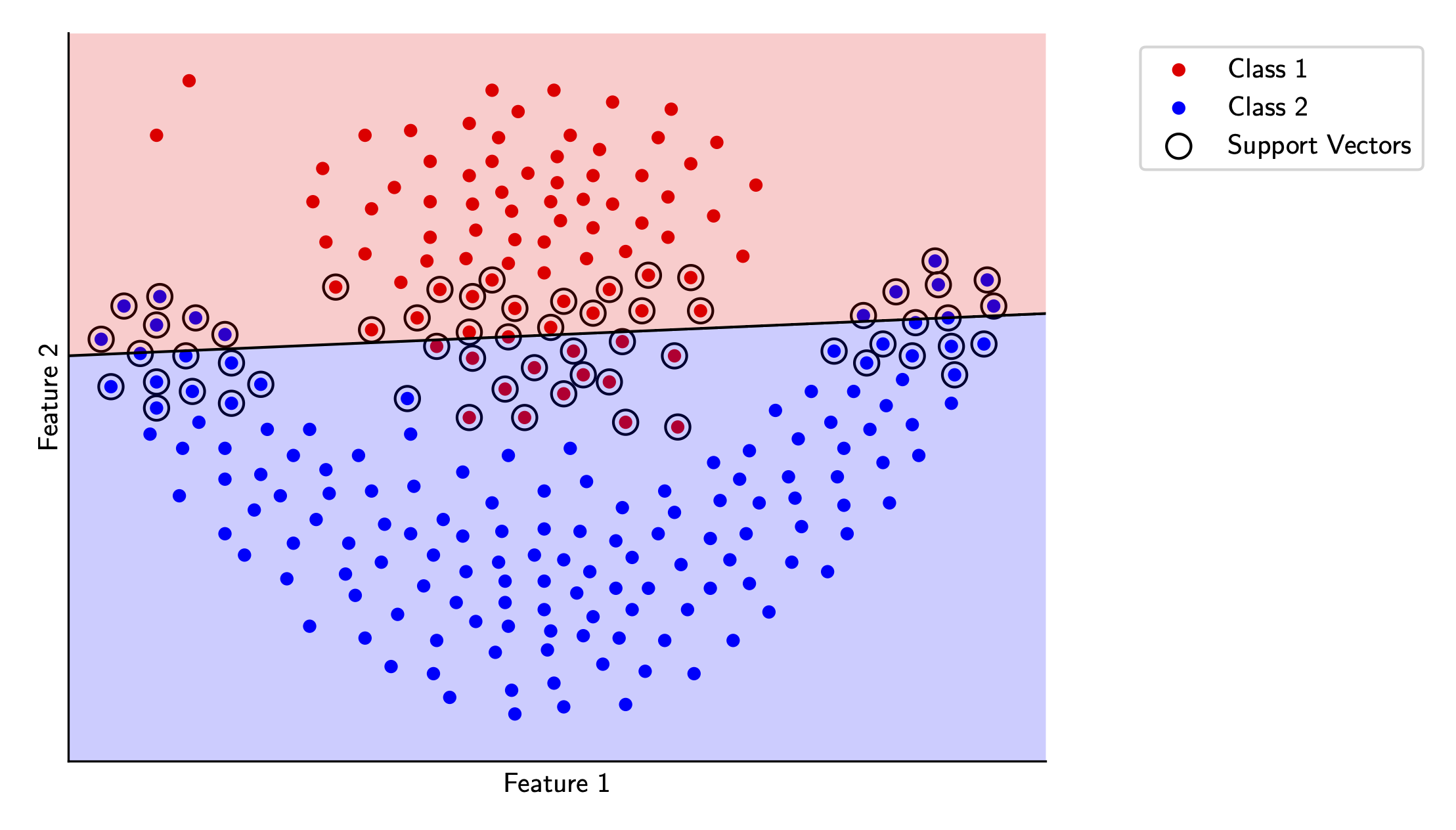
Here, I’ve also highlighted the support vectors for this decision boundary. You can see that most of the data actually doesn’t matter for the decision boundary, which is a neat feature of this type of classifier.
Kernels and Nonlinear Features
We’ve been through a lot of theory in the last section, yet our results on our toy dataset are still pretty mediocre with the SVM. The primary culprit for this is the fact that our decision boundary still has to be linear. For data such as is shown above, it’s impossible to classify every point accurately in this dataset in the input space shown without a non-linear decision boundary.
Let’s try and fix this issue. Remember our lifting trick from earlier? We turned data in \(d\)-dimensional space into \((d+1)\)-dimensional space by adding a constant bias term of \(1\) to each input sample. This was useful for the mathematics of the SVM, but we could feasibly add much more complex terms to our data instead of just one constant bias.
For example, let’s say we had data in two dimensions i.e. \(x = [x_1, x_2]\) and our decision boundary was some sort of ellipse i.e. \(f(x) = w_1x_1^2 + w_2x_2^2 + w_0\). A linear equation would never be able to model this decision boundary in the input space given. However, the equation of an ellipse is linear in some space - in this case the \(\tilde{x} = [x_1^2, x_2^2]\) space. Our decision boundary in this space is \(f(\tilde{x}) = w_1\tilde{x}_1 + w_2\tilde{x}_2 + w_0\), which is linear! Essentially, we’re applying a feature transformation \(\phi(x_1, x_2) \rightarrow (x_1^2, x_2^2)\) to our data, and finding a linear decision boundary in the transformed space instead of the original non-linear decision boundary.
Is this always possible? Surprisingly, yes, and the proof is almost trivial!
Suppose we have \(N\) points \(x_1 \dots, x_N\) and binary labels \(y_i \in \{−1,1\}\). Define a new feature mapping \(\phi(x_i) = e_i \in \mathbb{R}^N\) where \(e_i\) is the standard basis vector corresponding to \(i\), meaning it’s a vector of length \(N\) with all zeros except a \(1\) in the \(i\) -th position. Then, we can set \(w = (y_1, \dots, y_N)\), and \(f(\phi(x_i)) = w \cdot e_i = y_i\) for every sample \(i\), because each axis will only be active for it’s particular label.
This is the true power of linear classifiers - if we add non-linear features in our input space, we can essentially treat any type of classification problem (linear or non-linear) as a linear classification problem!
However, one might ask why we can’t just do the feature transformation I defined above for every dataset. The reason is that for a generic kernel transform, the time is takes to compute is generally \(\Omega(d)\). This isn’t practical because the process to compute the basis vectors scales linearly with the number of features, but it shows that there is always some higher dimensional space where the data is linearly separable.
However, for some transformations, we can compute the dot product \(\phi(x_i) \cdot \phi(x_j)\) much faster than we can compute the feature transformations individually. Let’s take a look at some practical examples of this feature transformation function \(\phi(x)\) (also called a kernel transformation) with this in mind.
First, let’s consider the quadratic kernel transform for data in \(\mathbb{R}^d\). For \(x = (x_1, \dots, x_d)\), we can compute the direct feature transform \[ \phi(x) = (x_1^2,\dots,x_d^2, \sqrt{2}x_1 x_2, \dots, \sqrt{2}x_{d-1}x_{d}, \dots, \sqrt{2}x_1, \dots, \sqrt{2} x_d, 1) \] in \(O(d^2)\) time.
However, the dot product ends up being quite nice \[ \begin{align*} \phi(x_1) \cdot \phi(x_2) &= \sum_{i=1}^{d} x_{1i}^2 x_{2, i}^2 + \sum_{1 \le i < j \le d} 2 \, x_{1i} x_{1j} \, x_{2i} x_{2j} + \sum_{i=1}^{d} 2 \, x_{1i} x_{2i} + 1\\ &= \left(\sum_{i=1}^d x_{1i}x_{2i} \right)^2 + 2 \sum_{i=1}^{d} x_{1i} x_{2i} + 1\\ &= \left(x_1 \cdot x_2\right)^2 + 2 \, (x_1 \cdot x_2) + 1 \end{align*} \] We can compute this in \(O(d)\) time, much faster than the \(O(d^2)\) time it would’ve taken to compute the feature map for each individually.
With this trick, we can even use infinite dimensional data! A common choice of kernel is the RBF (radial basis function) kernel i.e. \[ \phi(x) = \left(\frac{2}{\pi}^{\frac{d}{4}} \exp(- \lVert x - \alpha\rVert^2) \right)_{\alpha \in \mathbb{R}^d} \] The dot product is a bit involved but ends up being \(\phi(x_1) \cdot \phi(x_2) = \exp(-\lVert x_i - x_j \rVert^2)\), which we can compute in \(O(d)\). This is incredibly powerful, since it essentially allows us to process infinite-dimensional data in linear time!
Let’s take a look at the SVM optimization problem again. We have \[ \max_{0 \leq \alpha_i \leq C} \sum_{i=1}^n \alpha_i - \frac{1}{2} \sum_{i=1} \sum_{j=1} \alpha_i\alpha_jy_iy_j(x_i \cdot x_j) \] Notice that our optimization problem doesn’t depend on \(x_i\) or \(x_j\) individually, but only the dot product between them. This is the “nice” part of the dual formulation of the SVM problem - we can use any kernel transformation here to extend our SVM problem to non-linear features efficiently. Mathematically, for an arbitrary feature transform \(\phi(x)\), we can write the dual formulation as \[ \max_{0 \leq \alpha_i \leq C} \sum_{i=1}^n \alpha_i - \frac{1}{2} \sum_{i=1} \sum_{j=1} \alpha_i\alpha_jy_iy_j(\phi(x_i) \cdot \phi(x_j)) \] and choose \(\phi(x)\) to make the dot product computationally feasible to compute.
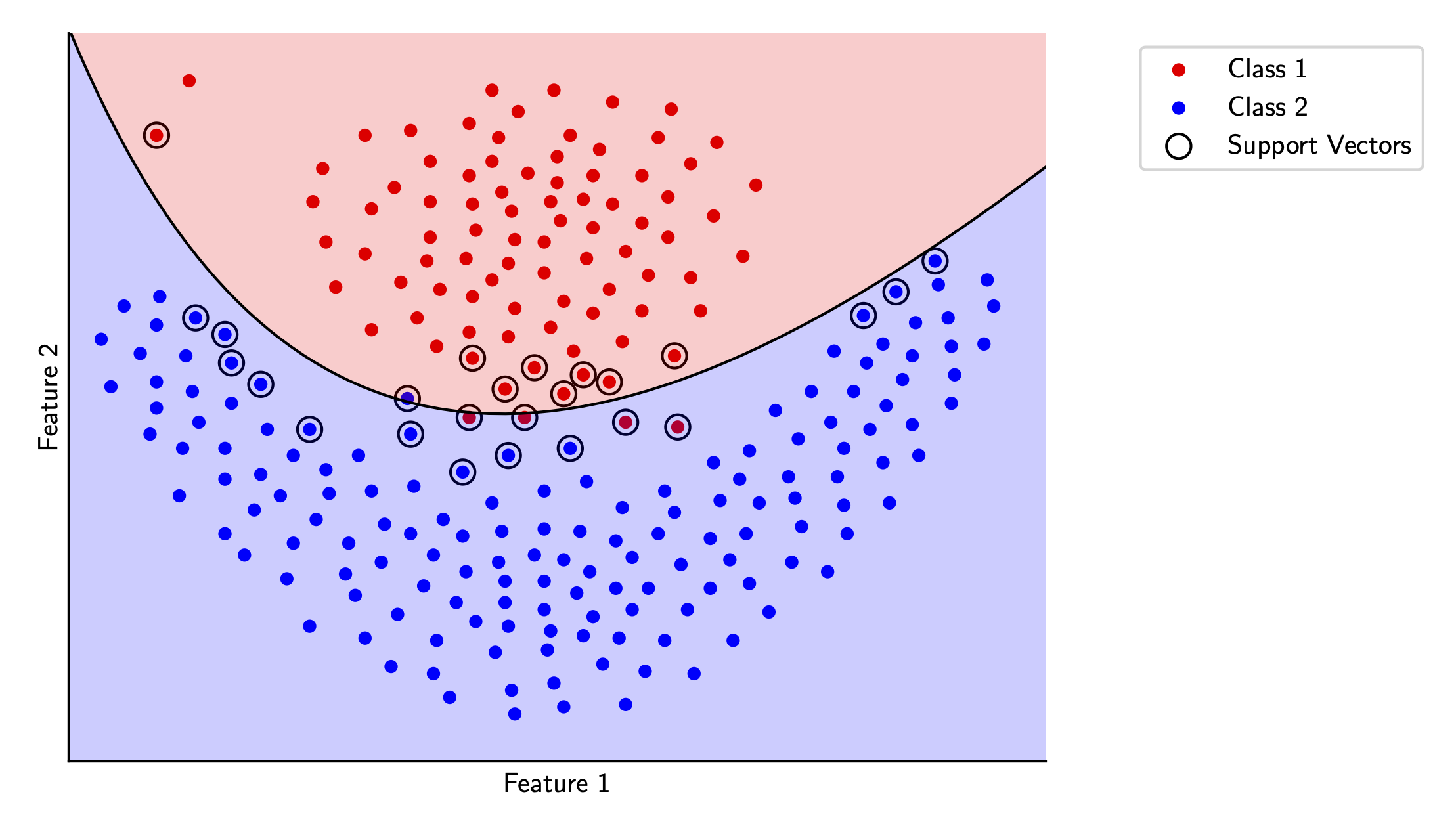
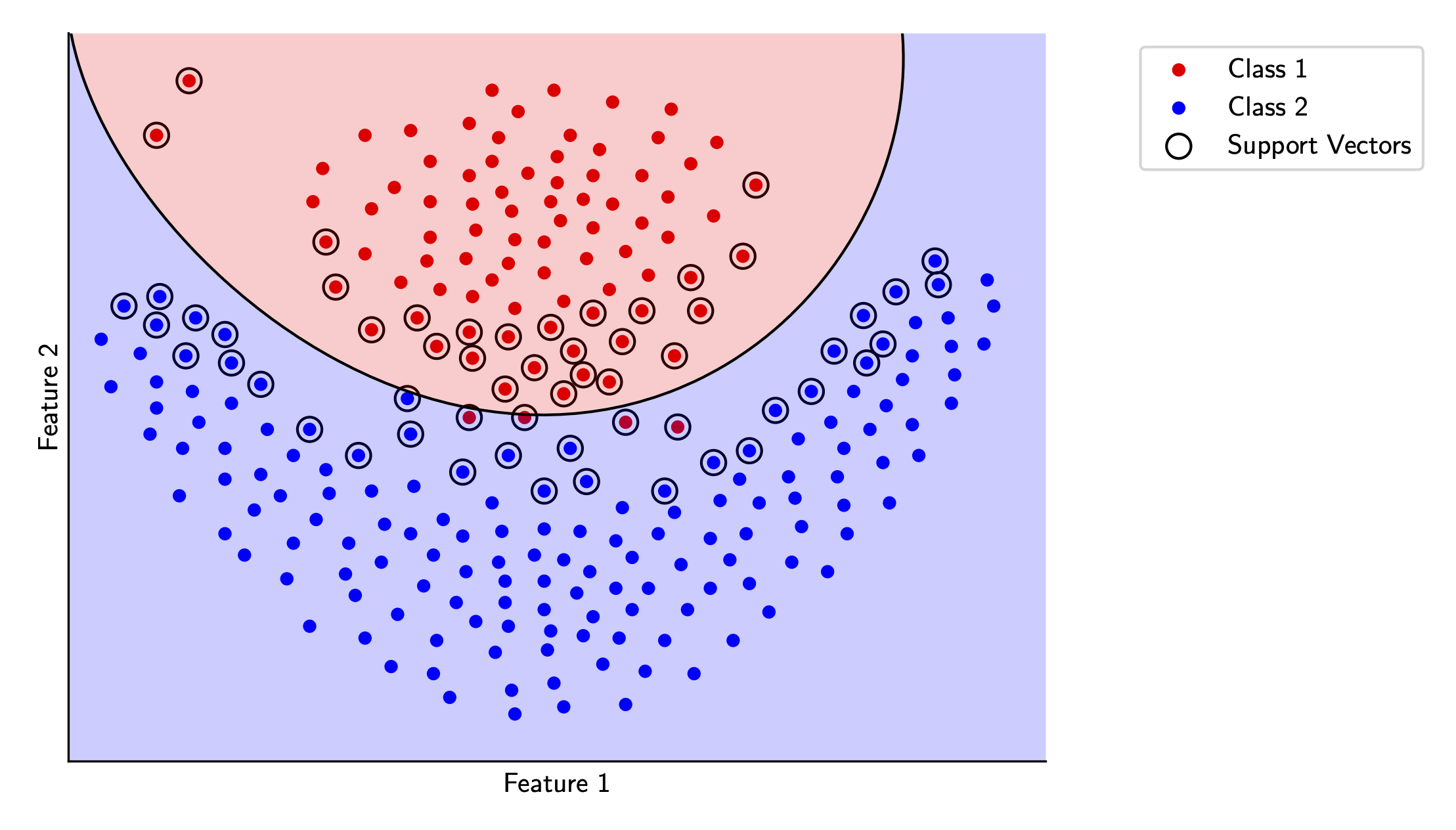
Let’s see how this works for our sample data. We’ll try out the polynomial kernel and the RBF kernel in scikit-learn and visualize each.
Again, all code for this article is available here.
Wrap-up
With that, our overview of linear classification is complete. There’s a ton of depth in this topic that I haven’t been able to cover here, but I hope this article served as a good overview, especially for the non-intuitive mathematical bits.
If you’ve made it this far, thank for reading through as always! For the next part of this series, I’ll dive deeper into a field we discussed in my first article in this series - that of regression.
All diagrams are made by me unless noted otherwise.