Machine Learning Fundamentals: Linear Classification (1/2)

---

Introduction

---

In my previous article, I covered supervised learning. Now, we’ll dive deeper into one of the topics covered in that article - namely, linear classification. This article is the first part of two - in this part, I’ll lay out a baseline understanding of classification problem in general as well as some useful techniques.

As from before, my goal with this series is to serve as an educational tool for those looking to review the fundamentals of machine learning with an emphasis on ease of understanding. This series assumes some familiarity with machine learning in general, and as such I will try to focus on the underlying mathematics and intuition behind the concepts that we discuss.

Linear Classification

---

As you may recall from last article, classification refers to a set of problems where the input is from a $d$ -dimensional set $\mathcal{X}$ , and the output is from a set of finite categorial values, which we will refer to as $\mathcal{Y}$ . A classifier will refer to a function $f(x)$ that outputs a label $y \in \mathcal{Y}$ for an input sample $x$ . We will train this classifier on input data $X$ and output labels $Y$ .

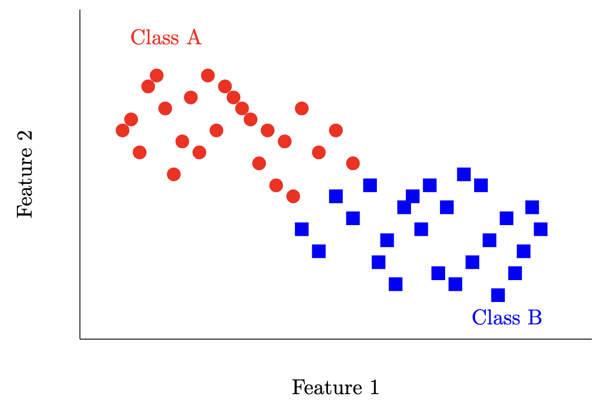
For example, for the dataset below, we’d like a function that can take in a sample point $x$ (here, $d = 2$ ) and output a label $y$ for either Class A (red) or Class B (blue). Usually, we’ll assign numbers to classes (i.e. Class A becomes 0, and Class B becomes 1) so we can write $y \in {0, 1}$ .

There are a few types of classifiers we could naively construct off the top of our heads. For example, the constant classifier $f(x) = y$ for some fixed $y \in \mathcal{Y}$ for all inputs $x \in \mathcal{X}$ (i.e. in the example above classify red for everything).

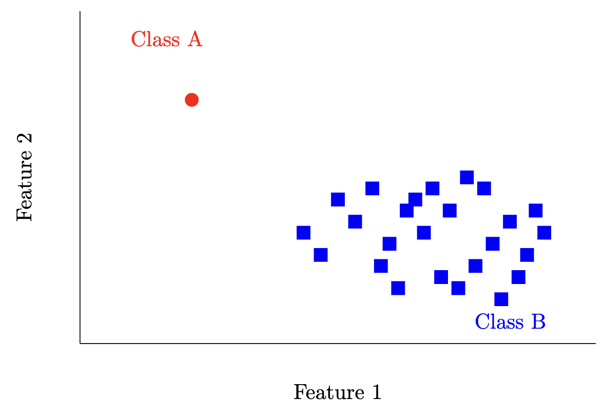
Another simple classifier would be the majority class classifier i.e. $f(x) = \argmax_{y \in \mathcal{Y}} P[Y = y]$ . There are definitely some datasets this could work really well for (see below), but in general we can do better.

Bayes Classifier

---

How much better? To answer that quantitatively, we’ll take a look at a classifier known as the Bayes classifier, which is defined rather simply:
$$f(x) = \argmax_{y \in \mathcal{Y}} P[Y = y | X = x]$$

As it turns out, this classifier is actually optimal! More formally, for an arbitrary classifier $g(x) = \mathcal{X} \to \mathcal{Y}$ , we can write
$$P_{x, y} [g(x) = y] \leq P_{x, y} [f(x) = y]$$
where $P_{x, y} [f(x) = y]$ is known as the accuracy of a classifier $f$ . Intuitively, you can just think of accuracy as the percentage of samples that a classifier labels correctly.

It’s understandable to be skeptical of this result - after all, why do we need all these fancy neural networks if the optimal classifier is this simple? Let’s first go over the proof of this result and then we can take a look at why this classifier isn’t practical.

Here, we’ll cover the proof of this result for binary $\mathcal{Y}$ i.e. the only classes are $0$ and $1$ for simplicity, although the proof does extend generally to the case of any number of categories.

Let’s consider an individual sample $x \in X$ . Then, for any classifier $h$ ,
$$\begin{align*} P[h(x) = y | X = x] &= P[h(x) = 1, Y = 1 | X = x] + P[h(x) = 0, Y = 0 | X = x]\\ &= \mathbf{1}[h(x) =1 ]P[Y = 1 | X = x] + \mathbf{1}[h(x) = 0 ]P[Y = 0 | X = x]\\ \end{align*}$$
Let’s let $\eta(x) = P[Y = 1 | X = x]$ . Then, we can write
$$P[h(x) = y | X = x] = \mathbf{1}[h(x) =1 ]\eta(x) + \mathbf{1}[h(x) = 0 ](1 - \eta(x))$$
Now, let’s use our original $f$ and $g$ again. We can write
$$\begin{align*} &P[f(x) = y | X = x] - P[g(x) = y | X = x]\\ &= \left(\mathbf{1}[f(x) =1 ]\eta(x) + \mathbf{1}[f(x) = 0 ](1 - \eta(x))\right) - \left(\mathbf{1}[g(x) =1 ]\eta(x) + \mathbf{1}[g(x) = 0 ](1 - \eta(x))\right) \\ &=\eta(x)\left(\mathbf{1}[f(x) =1 ] - \mathbf{1}[g(x) =1 ]\right) + (1 - \eta(x))\left(\mathbf{1}[f(x) = 0 ] - \mathbf{1}[g(x) = 0 ]\right)\\ &= \eta(x)(\mathbf{1}[f(x) = 1] - \mathbf{1}[g(x) = 1]) + (\mathbf{1}[f(x) = 0] - \mathbf{1}[g(x) = 0]) \\ &\quad - \eta(x)(\mathbf{1}[f(x) = 0] - \mathbf{1}[g(x) = 0]) \\ &= \eta(x)[(\mathbf{1}[f(x) = 1] - \mathbf{1}[g(x) = 1]) - (\mathbf{1}[f(x) = 0] - \mathbf{1}[g(x) = 0])] \\ &\quad + (\mathbf{1}[f(x) = 0] - \mathbf{1}[g(x) = 0]) \end{align*}$$
Here, we can use the fact that $\mathbf{1}[f(x) = 1] = 1 - \mathbf{1}[f(x) = 0]$ to simplify further.
$$\begin{align*} &\eta(x)\left[ (\mathbf{1}[f(x) = 1] - \mathbf{1}[g(x) = 1]) - ((1 - \mathbf{1}[f(x) = 1]) - (1 - \mathbf{1}[g(x) = 1])) \right] \\ &\quad + ((1 - \mathbf{1}[f(x) = 1]) - (1 - \mathbf{1}[g(x) = 1])) \\ &= \eta(x)[(\mathbf{1}[f(x) = 1] - \mathbf{1}[g(x) = 1]) - (-\mathbf{1}[f(x) = 1] + \mathbf{1}[g(x) = 1])] \\ &\quad + (-\mathbf{1}[f(x) = 1] + \mathbf{1}[g(x) = 1]) \\ &= 2\eta(x)(\mathbf{1}[f(x) = 1] - \mathbf{1}[g(x) = 1]) - (\mathbf{1}[f(x) = 1] - \mathbf{1}[g(x) = 1]) \\ &= (2\eta(x) - 1)(\mathbf{1}[f(x) = 1] - \mathbf{1}[g(x) = 1]) \end{align*}$$
Recall $\eta(x) = P[Y = 1 | X = x]$ . We now can consider three cases.

First, if $\eta(x) = \frac{1}{2}$ , it doesn’t matter what either classifier picks since the term $2\eta(x) - 1 = 0$ , so the entire expression will be $0$ .

Second, when $\eta(x) > \frac{1}{2}$ , the Bayes classifier will pick $1$ since $\eta(x) = P[Y = 1 | X = x] > P[Y = 0 | X = x]$ , which means $\mathbf{1}[f(x) = 1] = 1$ . If the arbitrary classifier selects $1$ for $x$ , the overall expression will be $0$ , and otherwise it will be positive. Mathematically, $(2\eta(x) - 1)(\mathbf{1}[f(x) = 1] - \mathbf{1}[g(x) = 1]) \geq 0$ when $\eta(x) > \frac{1}{2}$ .

Finally, when $\eta(x) < \frac{1}{2}$ , the Bayes classifier will pick $0$ since $\eta(x) = P[Y = 1 | X = x] < P[Y = 0 | X = x]$ , which means $\mathbf{1}[f(x) = 1] = 0$ . If the arbitrary classifier selects $0$ for $x$ , the overall expression will be $0$ , and otherwise it will still be positive, since $2\eta(x) - 1 < 0$ when $\eta(x) < \frac{1}{2}$ . Mathematically, $(2\eta(x) - 1)(\mathbf{1}[f(x) = 1] - \mathbf{1}[g(x) = 1]) \geq 0$ when $\eta(x) < \frac{1}{2}$ as well.

Therefore, this expression is always non-negative! What does this mean? Recall where we started from i.e. $P[f(x) = y | X = x] - P[g(x) = y | X = x]$ . We’ve shown that this is equal to $(2\eta(x) - 1)(\mathbf{1}[f(x) = 1] - \mathbf{1}[g(x) = 1])$ and furthermore that this is always non-negative, meaning we can write
$$\begin{align*} P[f(x) = y | X = x]& - P[g(x) = y | X = x] \geq 0\\ P[f(x) = y | X = x]& \geq P[g(x) = y | X = x] \end{align*}$$
or in other words, the accuracy of the Bayes classifier is greater than any arbitrary classifier for a fixed point $x$ . Our logic above didn’t depend on the particular choice of $x$ , meaning that the same logic applies to any point $x$ . Therefore, the Bayes classifier is optimal globally. A quick note here: optimal does not necessarily mean perfect, as shown below.

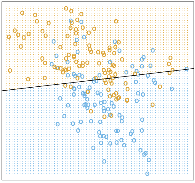
We’ve shown that the Bayes classifier cannot be beaten (as visualized above). Why then, do we need any of the items we’re about to discuss in this article? The answer lies in need for the conditional data distribution $P[Y | X]$ in the Bayes classifier.

Since the true data distribution is unknown, this data distribution is also unknown, meaning we need to estimate it from observed data samples. However, there can be infinite possible choices of $x \in \mathcal{X}$ meaning that the amount of data needed to estimate this is not practical, especially as the dimension of $\mathcal{X}$ increases. So although the Bayes classifier is optimal, it is generally unfeasible to directly model in practice, leading us find smarter routes.

Naive Bayes Classifier

---

Let’s take a look at the definition of the Bayes classifier again.
$$f(x) = \argmax_{y \in \mathcal{Y}} P[Y = y | X = x]$$
One way we can simplify this is by using Bayes’ rule i.e.
$$P (A | B) = \frac{P(B | A) P(A)}{P(B)}$$
Applying it here, we’ll get
$$\begin{align*} f(x) &= \argmax_{y \in \mathcal{Y}} P[Y = y | X = x]\\ &= \argmax_{y \in \mathcal{Y}} \frac{P[X = x | Y = y] P [Y = y]}{P[X = x]} \end{align*}$$
In our equation, since we are taking the $\argmax$ over all possible values of $y$ , and $P[X = x]$ is independent of $y$ , we can actually remove that term entirely and write
$$f(x) = \argmax_{y \in \mathcal{Y}} P[X = x | Y = y] P[Y = y]$$
Intuitively, this equation tells us that if we can estimate the probability that the input sample $x$ came from the class-conditional distribution $P[X = x | Y = y]$ , we can then weight this probability by the class prior (i.e. $P[Y = y]$ ), and choose the most likely class accordingly.

This is much more tractable than the original specification of the Bayes classifier, since we don’t need to estimate the full posterior distribution $P[Y = y | X = x]$ , and can instead estimate $|\mathcal{Y}|$ class-specific distributions $P[X = x | Y = y]$ and prior probabilities $P[Y = y]$ .

With this formulation, we have a lot of flexibility in terms of how we choose to model $P[X = x | Y = y]$ . If we assume that the data has some sort of form, we can choose to do some form of parametric density estimation. Essentially, we choose a type of model or distribution (i.e. linear, Gaussian, Bernoulli, etc.), and choose the parameters that are most likely to fit the given data. There are also non-parametric ways of estimating the distributions, which we may cover at another time.

One very simple way of estimating these distributions is add another assumption to our problem. If we assume that individual features are independent given the class label, we can split out the $d$ -dimensional $x$ into probabilities for each of the $d$ features. This classifier is known as the Naive Bayes Classifier.

$$f(x) = \argmax_{y \in \mathcal{Y}} \prod_{j=1}^d P[X_j = x_j | Y = y] P[Y = y]$$
This is a very simple model to implement in practice. However, because of the assumption of independence between features (which is generally not true), this classifier tends to result in bad estimates.

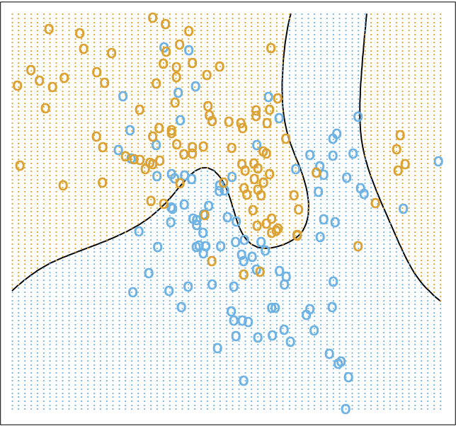
A very common choice in practice is to fit a Gaussian distribution for each class, parameterized by class specific means and variances. This is a common choice of class-conditional distribution due to the nice properties the Gaussian distribution has, especially as we increase the dimensionality of our problem. Let’s visualize what this classifier might look like for our toy example from earlier.

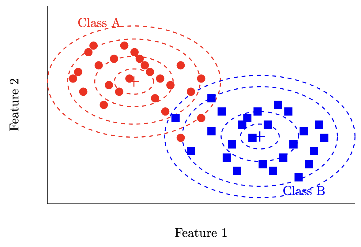
This classifier also allows us to measure our confidence in our prediction for each sample we classify per class, which is very useful for certain applications.

Maximum Likelihood Estimation

---

A reasonable question to ask at this point would be how we actually fit models like the one mentioned above to the data we have been given (as well as how any of this relates to linear classification). Rest assured, we’re slowly getting there - in this section we’ll tie all these concepts together through our discussion of maximum likelihood estimation.

Maximum likelihood estimation (MLE) is a technique used to estimate the parameters of a model to some set of data. First, let’s assume we have some data $X \sim \mathcal{X}$ , and that each sample $x \in X$ is independent and identically distributed (i.i.d) (this last assumption is important for later!). Then, let’s say we want to fit some class of parameterized models $\mathcal{P} = \{p_\theta | \theta \in \Theta\}$ , where each model $p$ can be uniquely described by a set of parameters $\theta$ from the set of all possible parameter choices $\Theta$ .

We define the likelihood function as follows
$$\mathcal{L}(\theta | X) = P(X | \theta) = \prod_{i=1}^n P(x_i | \theta) = \prod_{i=1}^n p_\theta(x_i)$$
where the second to last step is possible because of our i.i.d. assumption from earlier. Intuitively, this function represents how probably (or likely) is the data given the model $p_\theta$ . Maximum likelihood estimation then simply becomes which parameter setting maximizes the likelihood function, or mathematically
$$\argmax_{\theta} \mathcal{L}(\theta | X) = \argmax_{\theta} \prod_{i=1}^n p_\theta(x_i)$$

With this new formulation, let’s take a look at a toy example where we model our class conditional distributions with univariate Gaussians. Recall the probability density function for the Gaussian distribution
$$p_{\{\mu, \sigma^2\}}(x) = \frac{1}{\sqrt{2\pi\sigma^2}} \exp \left(- \frac{(x - \mu)^2}{2\sigma^2}\right)$$
Then, our MLE problem becomes
$$\argmax_{\theta} \mathcal{L}(\theta | x) = \argmax_{\mu, \sigma^2} \prod_{i=1}^n p_{\{\mu, \sigma^2\}}(x_i)$$
There are two tricks we can use here to make this problem a little easier. First, since the logarithm function is strictly monotonically increasing for non-negative values, we know that
$$\argmax_{\theta} \mathcal{L}(\theta | x) = \argmax \log \mathcal{L}(\theta | x)$$
Therefore, instead of our earlier equation, we have
$$\begin{align*} \argmax_{\theta} \mathcal{L}(\theta | x) &= \argmax \log \mathcal{L}(\theta | x) \\ &= \argmax_{\mu, \sigma^2} \log \prod_{i=1}^n p_{\{\mu, \sigma^2\}}(x_i)\\ &= \argmax_{\mu, \sigma^2} \sum_{i=1}^n \log p_{\{\mu, \sigma^2\}}(x_i) \end{align*}$$
which is a lot nicer to analyze than the nasty product we had before.

The second trick is one you’re probably familiar with from high school calculus - namely, that finding the maximum or minimum of a function boils down to analyzing it’s stationary points, which are values when the derivative of the function is zero.

Let’s take a look at the derivative of $\sum_{i=1}^n \log p_{\{\mu, \sigma^2\}}(x_i)$ with respect to $\mu$ and $\sigma^2$ respectively. First, let’s simplify the inner expression. We can write
$$\log p_{\{\mu, \sigma^2\}}(x_i) = -\frac{1}{2}\log(2\pi\sigma^2) - \frac{(x_i - \mu)^2}{2\sigma^2}$$

Then, to find our MLE estimate of $\mu$ , we have
$$\begin{align*} 0 &= \nabla_\mu \left(\sum_{i=1}^n \left[-\frac{1}{2}\log(2\pi\sigma^2) - \frac{(x_i - \mu)^2}{2\sigma^2}\right] \right)\\ &= \sum_{i=1}^n \nabla_\mu \left(-\frac{1}{2}\log(2\pi\sigma^2) - \frac{(x_i - \mu)^2}{2\sigma^2}\right)\\ &= \sum_{i=1}^n \left[\nabla_\mu \left(-\frac{1}{2}\log(2\pi\sigma^2)\right) - \nabla_\mu\left(\frac{(x_i - \mu)^2}{2\sigma^2}\right)\right]\\ \end{align*}$$
We can discard the $\nabla_\mu \left(-\frac{1}{2}\log(2\pi\sigma^2)\right)$ term since there is no $\mu$ involved. Continuing on, we have
$$\begin{align*} 0 &= \sum_{i=1}^n \nabla_\mu\left(-\frac{(x_i - \mu)^2}{2\sigma^2}\right)\\ &= -\frac{1}{2\sigma}\sum_{i=1}^n \nabla_\mu [(x_i - \mu)^2]\\ &= -\frac{1}{2\sigma} \sum_{i=1}^n -2(x_i - \mu)\\ &= \frac{1}{\sigma} \sum_{i=1}^n (x_i - \mu) \end{align*}$$
We can then discard the constant $\frac{1}{\sigma}$ since we’re setting the expression to $0$ anyways and solve
$$\begin{align*} \sum_{i=1}^n (x_i - \mu) &= 0\\ -n\mu + \sum_{i=1}^n x_i &= 0\\ -n\mu + \sum_{i=1}^n x_i &= 0\\ \sum_{i=1}^n x_i &= n\mu\\ \mu_{MLE} &= \frac{1}{n}\sum_{i=1}^n x_i \end{align*}$$
Intuitively, the best estimate of the mean parameter for the class conditional distribution is the mean of all the samples in that class in our training data - pretty simple if you think about it, but it’s nice to show it mathematically.

Now for $\sigma^2$ (phew, here we go)
$$\begin{align*} 0 &= \nabla_{\sigma^2} \left(\sum_{i=1}^n \left[-\frac{1}{2}\log(2\pi\sigma^2) - \frac{(x_i - \mu)^2}{2\sigma^2}\right] \right)\\ &= \sum_{i=1}^n \nabla_{\sigma^2} \left(-\frac{1}{2}\log(2\pi\sigma^2) - \frac{(x_i - \mu)^2}{2\sigma^2}\right)\\ &= \sum_{i=1}^n \left[\nabla_{\sigma^2} \left(-\frac{1}{2}\log(2\pi\sigma^2)\right) - \nabla_{\sigma^2} \left(\frac{(x_i - \mu)^2}{2\sigma^2}\right)\right]\\ &= \sum_{i=1}^n \left[-\frac{1}{2\sigma^2} + \frac{(x_i - \mu)^2}{2\sigma^4}\right]\\ &= \sum_{i=1}^n \left[\frac{(x_i - \mu)^2 - \sigma^2}{2\sigma^4}\right]\\ \end{align*}$$
We can ignore the denominator out since we want the entire expression to be $0$ . We have
$$\begin{align*} 0 &= \sum_{i=1}^n \left[ (x_i - \mu)^2 - \sigma^2\right]\\ n\sigma^2 &= \sum_{i=1}^n (x_i - \mu)^2\\ \sigma^2_{MLE} &= \frac{1}{n}\sum_{i=1}^n (x_i - \mu)^2\\ \end{align*}$$

We have the MLE estimates for each class-conditional distribution now - we can just assume a Bernoulli distribution for the class priors (i.e. $P[Y = y]$ is just the fraction of samples with that label) and we’re done!

A small confession - the analysis I did above was for a univariate Gaussian, but in our case our data would require a multivariate Gaussian. Rest assured, the derivation ends up being essentially the same barring some complications associated with vector calculus - for the multivariate Gaussian defined as
$$p_{\mu, \Sigma}(x) = \frac{1}{\sqrt{(2\pi)^d|\Sigma|}}\exp\left(-\frac{1}{2}(x-\mu)^T\Sigma^{-1}(x-\mu)\right)$$
we’d have
$$\mu_{MLE} = \frac{1}{n}\sum_{i=1}^n x_i$$ $$\Sigma_{MLE} = \frac{1}{n}\sum_{i=1}^n (x_i - \mu_{MLE})(x_i - \mu_{MLE})^T$$

Implementation

---

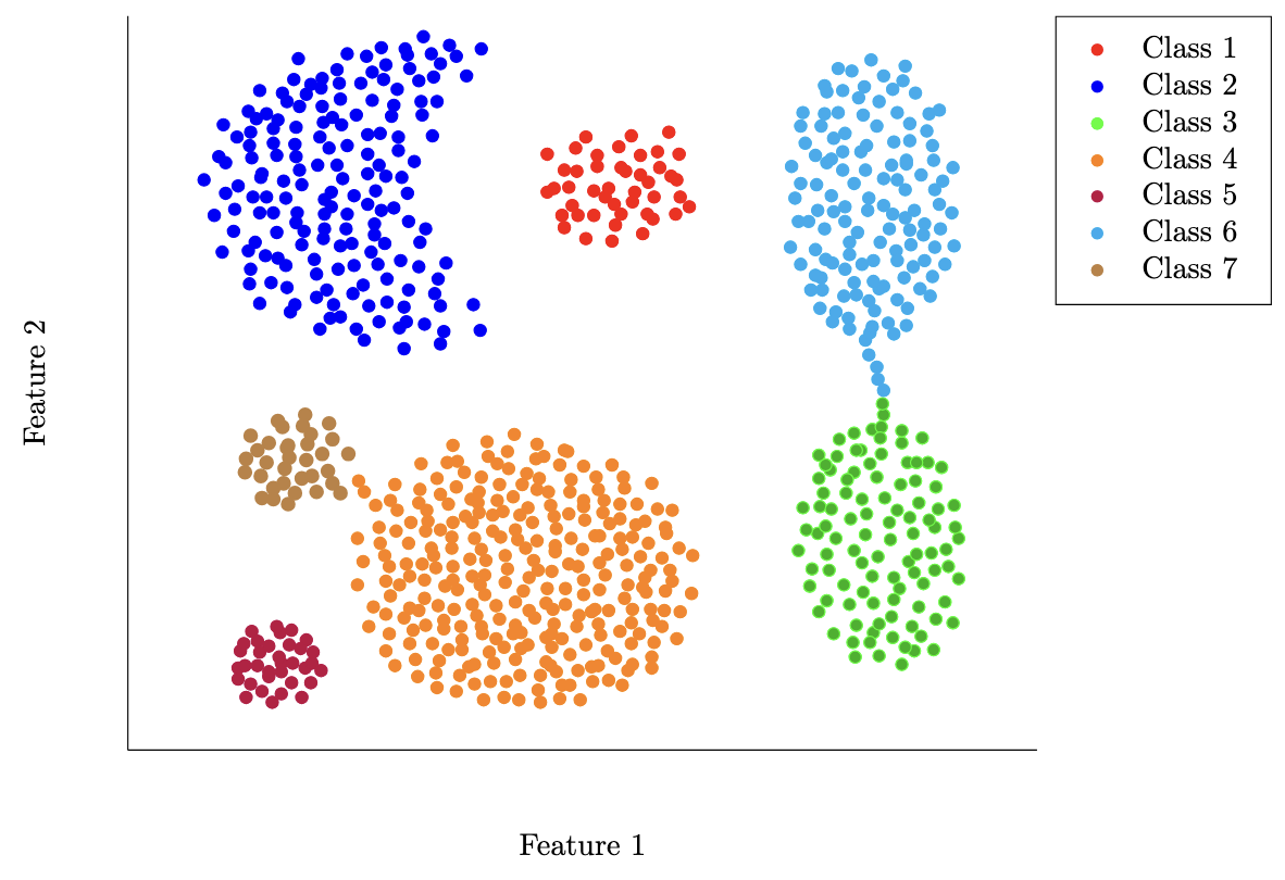
Our work has all been very theoretical up until now. For the remainder of the article, we’ll take a look at some toy examples based off this Kaggle dataset. I’ll include some small code snippets to show how you might implement these algorithms in practice. Let’s first visualize our dataset.

We can now write a function based off our derivations above to compute the class means and covariance matrices.

        
import pandas as pd
import numpy as np

CLASSES = np.sort(df['class'].unique())
CLASSES

def  fit_gaussian_mle(df):
    mle_params = {}

    for c in CLASSES:
        # get class data
        class_data = df[df['class'] == c]
        X = class_data[['feature1',  'feature2']].values

        # computed for classification, but not necessary to compute class means and variance
        p_y = len(class_data) / len(df)

        # mle parameter estimate for class mean
        mu_mle = np.mean(X, axis=0)

        # mle parameter estimate for class variance
        sigma_mle = np.zeros((len(X[0]),  len(X[0])))

        n = X.shape[0]
        X_centered = X - mu_mle # (x_i - mu)

        for i in  range(n):
            x_c_i = X_centered[i]
            x_c_i = x_c_i.reshape(-1,  1)  # make it a column vector
            sigma_mle += x_c_i @ x_c_i.T # (x_i - mu) * (x_i - mu)^T
        sigma_mle = sigma_mle / n # multiply by 1/n

        mle_params[int(c)] = {
            'mu': mu_mle,
            'sigma': sigma_mle,
            'prior': p_y
        }

    return mle_params

fit_gaussian_mle(df)

In my code above, I’ve refrained from using numpy functions like np.cov to be more clear with how our derivations end up being implemented in code. With the means and covariance matrices derived from this code, we can visualize our data as follows

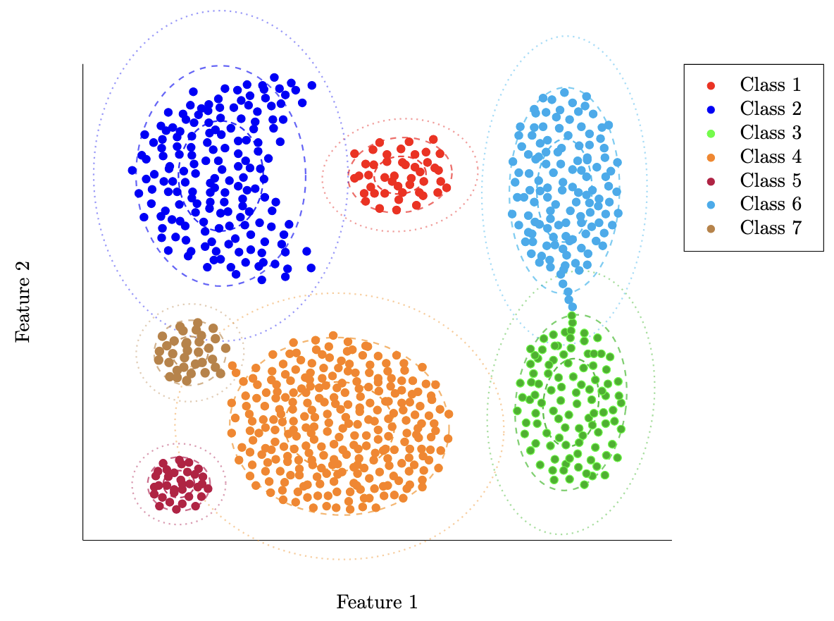
As you can see, in addition to classification, we are also able to plot ellipses showing the relative likelihood of each class the further we get from the mean of that class. In the cases where we have overlap, we’ll rely on the $\argmax$ feature of our original classifier to simply choose the class with the highest probability at that point.

Wrap-up

---

In this article, we’ve covered the basics of the classification problem, including topics such as the theory of the Bayes classifier and Maximum Likelihood Estimation. We also fit a sample dataset with MLE assuming Gaussian conditional distributions and demonstrated how you might implement this simple model in code.

If you’ve made it this far, thank for reading through as always! We’ve set up a baseline understanding of the world of classification in this article. Next time, I’ll dive more into linear classification itself, building up from the concepts we’ve covered this time.

All diagrams are made by me unless noted otherwise.

---