Siddarth Ijju

Machine Learning Fundamentals: Supervised Learning

Introduction

My goal with this series is to serve as an educational tool for those looking to review the fundamentals of machine learning with an emphasis on ease of understanding. This series assumes some familiarity with machine learning in general - for a more comprehensive introduction to the field, I’d recommend some online courses like this one. In addition, these articles will be less focused on the coding side of things and instead focus on the underlying mathematics and intuition behind these concepts.

To start, this article will cover supervised learning.

Supervised Learning

Many machine learning problems you can imagine begin with three components. First, there is a set of variables that are already measured or preset - this is commonly referred to as the input and is commonly notated with the symbol $X$ . These inputs have some influence on a set of variables known as the output, commonly denoted $Y$ . If you’ve taken a science class in high school, you may be more familiar with the terms independent variables and dependent variables - these refer to $X$ and $Y$ respectively.

Supervised learning refers to problems where you are given data with both these variables.

Classification vs Regression

There are generally two different types of measurements you can take for these variables. A quantitative measurement generally follows the patterns we associate with numerical values - for example, the price of a stock on a particular day. In contrast, you could also take a qualitative measurement - for example, what kind of animal you would be most likely to adopt. In the latter case, we assume the measurement can take values only from a finite set (i.e. there are not infinite types of animals in the world). Measurements like these are often referred to as categorical or discrete.

We can absolutely imagine problems of both types - given the salary of a homeowner, predict the square footage of their house, or given the grayscale values for the pixels of a digitized image of an animal, predict its class label. This distinction in output type has led to a naming convention for the types of problems they represent - classification refers to predicting qualitative outputs, and regression refers to predicting quantitative outputs.

The input type can also of course be either qualitative or quantitative, and there are techniques to handle both. In general, machine learning methods will tend to assume or be better suited for a certain type of input, with a few exceptions.

In practice, a computer does not have an understanding of qualitative concepts such as a species of animal or a type of feeling. As such, qualitative variables are often represented by codes - for example, cat = $0$ , dog = $1$ , etc. When there are only two cases, this is often referred to as a binary variable, since it can only take on the values of $0$ and $1$ . When there are more than two cases, it is also possible to represent a qualitative variable that can take on $k$ different values as a vector of $k$ binary variables, of which only the $k$ th variable is $1$ . This is referred to as one-hot encoding, and is useful because it is symmetric for all positions of $k$ as opposed to the actual numerical value of $k$ .

Linear Models and Least Squares

We can roughly state the learning task as follows: given an input $X$ , make a prediction of the output $Y$ , denoted by $\hat{Y}$ . The thing that does this for us is called a model. One of the simplest possible models used in machine learning is called the linear model, which is defined as follows.

Given a vector of inputs $X^T = (X_1, \dots X_p)$ for some finite $p$ , let’s assume the output $Y$ can be modeled linearly i.e. via a line. If we had one input, this equation will be familiar: $y = mx + b$ . For our vector-valued inputs and outputs, we predict the output $Y$ via the model

$\hat{Y} = \hat{\beta_0} + \sum_{j=1}^p X_j\hat{\beta_j}$
where the hat symbols are included to signify that there are predicted values. One common quality of life inclusion is to add a new constant feature of $1$ to $X$ , in which case we can include the constant $\hat{\beta_0}$ in a vector of coefficients $\hat{\beta}$ and write the linear model in vector form as

$\hat{Y} = X^T\hat{\beta}$

If both $X$ and $Y$ had only one dimension, the set $(X, \hat{Y})$ would represent a line in two dimensional space. In many cases however, $X$ and $Y$ have many dimensions - the equation above still works, but the set $(X, \hat{Y})$ in that case represents a hyperplane. For the following, we’ll assume that $X$ has $p$ dimensions and $Y$ has only one.

There are many different methods to fit the linear model to the training data, but one of the most popular is the least squares approach, in which we pick the coefficients of the vector $\beta$ to minimize the residual sum of squares over the $N$ training samples i.e.
$RSS(\beta) = \sum_{i=1}^N (y_i - x_i^T\beta)^2$
If we let $\bold{X}$ represent an $N \times p$ matrix with each row representing an input vector, and $\bold{y}$ is a vector of the $N$ training outputs, there is also a nice way to write this in vector notation as
$RSS(\beta) = (\bold{y} - \bold{X}\beta)^T(\bold{y} - \bold{X}\beta)$
We’d like to minimize $RSS(\beta)$ , so let’s take the gradient of this expression (let’s use the first one for simplicity) with respect to $\beta$ . We have
$\begin{align*} \frac{\partial}{\partial \beta}RSS(\beta) &= \frac{\partial}{\partial \beta} \sum_{i=1}^N (y_i - x_i^T\beta)^2 \\ &=\sum_{i=1}^N \frac{\partial}{\partial \beta} (y_i - x_i^T\beta)^2 \\ &=\sum_{i=1}^N -2(y_i - x_i^T\beta)x_i\\ &= -2\bold{X}^T(\bold{y} - \bold{X}\beta) \end{align*}$
where we convert to vector form at the least step. Setting this to zero and dropping the constant, we have
$\bold{X}^T(\bold{y} - \bold{X}\beta) = 0$

Linear Algebra Detour

Let’s try and solve this for $\beta$ - we have
$\begin{align*} \bold{X}^T(\bold{y} - \bold{X}\beta) &= 0\\ \bold{X}^T\bold{y} - \bold{X}^T\bold{X}\beta &= 0\\ \bold{X}^T\bold{y} &= \bold{X}^T\bold{X}\beta \end{align*}$
at which point we’re kind of stuck. Normally, we’d divide by $\bold{X}^T\bold{X}$ - in matrix mathematics this means we’d multiply by $(\bold{X}^T\bold{X})^{-1}$ . In general, we aren’t guaranteed that $\bold{X}^T\bold{X}$ is invertible, so we’ll have to find another avenue.

Luckily, we aren’t the first the have this issue - the Moore-Penrose inverse of a matrix $A$ (denoted by $A^{\dagger}$ ) was developed for this purpose. Also called the pseudoinverse, $A^{\dagger}$ is an approximation of the inverse of a matrix, in the sense that $A^{\dagger}$ exists even if the original matrix isn’t square or invertible.

Let’s take a quick detour and derive $A^{\dagger}$ from scratch, starting from the singular value decomposition (SVD) of $A$ . In my opinion, the SVD is where most of the magic happens for the pseudoinverse, and would be worth a whole post on its own - it is too in-depth for this article, but if you’d like a quick overview, I found this video very helpful.

Per SVD, we can write a matrix $A$ as $U\Sigma V^T$ , where $U$ is an orthogonal matrix whose columns are the left singular vectors of $A$ , $V$ is an orthogonal matrix whose columns are the right singular vectors of $A$ , and $\Sigma$ is a diagonal matrix containing the singular values of $A$ . Let’s say we’re trying to find a solution for $x$ in the system $Ax = b$ for some $b$ .

Since $U$ and $V$ are orthogonal when $A$ is real-valued (which is assumed), their inverses $U^{-1}$ and $V^{-1}$ are equivalent to $U^T$ and $V^T$ respectively. The inverse of $\Sigma$ is pretty easy to compute since it is diagonal - just construct a diagonal matrix with the reciprocal of all non-zero values in $\Sigma$ . As such, we can solve the system $Ax = b$ as follows

$\begin{align*} Ax &= b\\ U\Sigma V^T x &= b\\ V\Sigma^{-1}U^TU\Sigma V^T x &= V\Sigma^{-1}U^Tb\\ V\Sigma^{-1}(I)\Sigma V^T x &= V\Sigma^{-1}U^Tb\\ V(\Sigma^{-1}\Sigma) V^T x &= V\Sigma^{-1}U^Tb\\ V(I) V^T x &= V\Sigma^{-1}U^Tb\\ (VV^T) x &= V\Sigma^{-1}U^Tb\\ \tilde{x} &= V\Sigma^{-1}U^Tb\\ \end{align*}$
where the tilde in the last step denotes that this $x$ is not an exact solution for the original equation but rather an approximation. Therefore, for a matrix $A$ with a SVD of $U\Sigma V^T$ , the pseudoinverse can be defined $A^{\dagger} = V\Sigma^{-1}U^T$ .

Going back to our original problem, we can use the pseudoinverse to find a solution when $X^TX$ isn’t invertible, which results in the following general solution for linear least squares regression.

$\begin{align*} \bold{X}^T\bold{X}\beta &= \bold{X}^T\bold{y} \\ (\bold{X}^T\bold{X})^{\dagger}(\bold{X}^T\bold{X})\beta &= (\bold{X}^T\bold{X})^{\dagger}\bold{X}^T\bold{y}\\ \hat{\beta} &= (\bold{X}^T\bold{X})^{\dagger}\bold{X}^T\bold{y} \end{align*}$

With this, we’ve arrived at a solution for $\hat{\beta}$ that minimizes the residual sum of squares for our linear model $\hat{Y} = X^T\hat{\beta}$ . While this model is very simple to train (an analytical solution exists) and doesn’t require much data, it is still quite simplistic at its core. One can visualize many datasets that may not align well with a linear decision boundary, such as in the image below. Here, the values for $Y$ are assigned to $0$ or $1$ to represent a classification and we can plot $\{x: x^T\hat{\beta}\}$ , which is the decision boundary that separates the two classes.

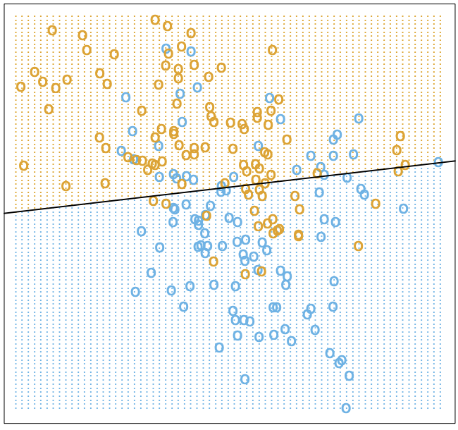
Even in the ideal case, we can end up misclassifying many potential points for both classes. When this happens, one possible thing to try is a different model that may be better suited for the task at hand, which is what we will take a look at next.

Nearest Neighbors

There is a saying that “birds of a feather flock together”, or in more colloquial terms, that things or people of the same sort will be found together. This is the general concept behind our next model, known as the nearest neighbors method.

Formally, nearest neighbors methods will use the observations in the training set $\mathcal{T}$ that are “closest” to an input sample $x$ to form $\hat{Y}$ . For a given $k$ , we can write this as
$\hat{Y}(x) = \frac{1}{k} \sum_{x_i \in N_k(x)} y_i$
where $N_k(x)$ represents the neighborhood of $x$ defined by the $k$ “closest” points. Intuitively, this equation simply says that the predicted label or value for a sample $x$ will be the average of the $k$ “closest” samples in the training data.

“Closest” isn’t strictly defined in our setting yet, which is why I’ve put it in quotes so far. There are many metrics one could use to define the distance of one vector to another, but in practice the most commonly used metric is Euclidean distance. Some others include cosine distance or Hamming distance, useful for high dimensional data and categorical data respectively.

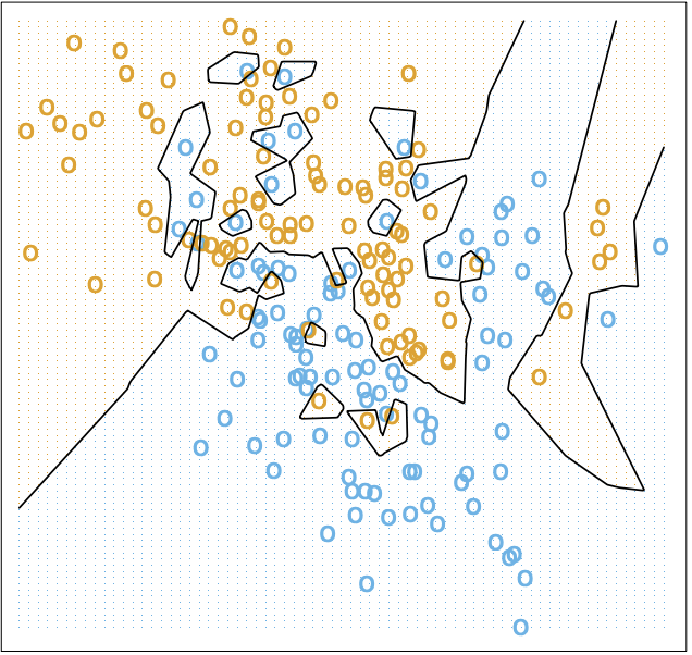
You can see how this works for $k=1$ below. For lower values of $k$ , since the label is defined by fewer neighbors, the decision boundary would be more jagged, which is corroborated below.

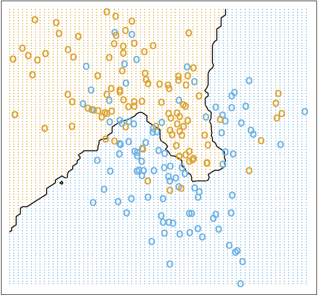
1-Nearest Neighbors — (from *The Elements of Statistical Learning, Section 2*)

For higher values of $k$ , the decision boundary becomes much smoother, as you can see. The choice of $k$ is often included as a hyperparameter in the nearest neighbor model (a hyperparameter more generally refers to a model setting that is set before the model is trained).

k-Nearest Neighbors — (from *The Elements of Statistical Learning, Section 2*)

As you can see, choosing $k$ is not so easy as minimizing the residual sum of squares, like we did for the linear model above. At $k=1$ , we have zero error on the training set, so the residual sum of squares approach would always yield that - however, this is clearly not the most generalizable or desirable model for our data.

Similar to the linear model, the nearest neighbors model requires little training. One drawback of the model however, is the need to maintain the training dataset in memory every time we want to make an inference. For smaller datasets, this can be acceptable but as we scale our datasets up this will become more and more of a problem.

Although I won’t go into it in this article, several methods do exist to make nearest neighbors more efficient - for example, you could store the points in an efficient structure such as a k-d tree and only keep points up to a certain level in the tree. You could also use a locality sensitive hashing method, where you hash points into buckets based on their distance from each other to compress the necessary data. If we only cared about classification, we could also compute means for each of the $\frac{N}{k}$ neighborhoods, and at inference simply give the label of the neighborhood whose mean is closest to the input. All these methods trade accuracy for scalability, which is a common trend you will see in the machine learning field in general.

Bias-Variance Tradeoff

We’ve seen some patterns in the simple linear models we’ve outlined above. Without losing generality, we can observe for the toy example above that the linear model is more “stable” but less “accurate” overall, while the nearest neighbors model is more “accurate” but less “stable”. We can formalize this intuition through a concept known as the bias-variance tradeoff.

For both our models above, we have a hypothesis $h(x)$ that generates our prediction $\hat{y}$ for our individual input $x$ . We can decompose the error our hypothesis function $h(x)$ to fit the ground truth function $g(x)$ into two terms.

First is the bias. The bias represents error caused by the inability of the hypothesis $h$ to fit $g$ perfectly. For example, if we picked a linear hypothesis $h$ to fit a quadratic function $g$ , the error caused by the discrepancy in model choice would result in a higher bias.

Second is the variance. The variance represents error caused by fitting random noise in the training data i.e. even if we do pick a linear model $h$ to match a linear model $g$ , the difference $h(x) - g(x)$ would be attributed to variance.

Let’s assume we are fitting a model $h(x)$ to inputs sampled from a distribution $D$ and noise (notated as $\epsilon$ ) sampled from a distribution of the same shape $D'$ . We can write $X_i \sim D$ , $\epsilon_i \sim D'$ and $y_i = g(X_i) + \epsilon_i$ .

Let’s take a look at the expected squared error for an arbitrary point $z$ . Our “true” label in our dataset can be written as $\gamma = g(z) + \epsilon, \epsilon \sim D'$ , since we can’t remove the noise that would be present in our training dataset. We can then write the expected squared error as
$\begin{align*} \mathbb{E}[(h(z) - \gamma)^2] &= \mathbb{E}[h(z)^2 - 2h(z)\gamma + \gamma^2]\\ &= \mathbb{E}[h(z)^2] - 2\mathbb{E}[h(z)\gamma] + \mathbb{E}[\gamma^2] \end{align*}$
Recall $Var(X) = \mathbb{E}[X^2] - \mathbb{E}[X]^2$ for a random variable $X$ . Additionally, since $h(z)$ and $\gamma$ are independent, we can then write
$\begin{align*} \mathbb{E}[(h(z) - \gamma)^2] &= \mathbb{E}[h(z)^2] + \mathbb{E}[\gamma^2] - 2\mathbb{E}[h(z)\gamma] \\ &= \left(Var(h(z)) + \mathbb{E}[h(z)]^2\right) + \left(Var(\gamma) + \mathbb{E}[\gamma]^2\right) - 2\mathbb{E}[h(z)]\mathbb{E}[\gamma]\\ &= Var(h(z)) + Var(\gamma) + \mathbb{E}[h(z)]^2 - 2\mathbb{E}[h(z)]\mathbb{E}[\gamma] + \mathbb{E}[\gamma]^2 \\ &= \left(\mathbb{E}[h(z)] - \mathbb{E}[\gamma]\right)^2 + Var(h(z)) + Var(\gamma) \\ \end{align*}$
This is known as the bias-variance decomposition. The term $\left(\mathbb{E}[h(z)] - \mathbb{E}[\gamma]\right)^2$ represents the bias, intuitively just the squared error between the expected prediction and the expected ground truth. The term $Var(h(z))$ is the variance of the hypothesis prediction. Finally, the term $Var(\gamma)$ represents the irreducible error of the model, which is essentially the error caused by noise in the labels of the training dataset.

With this, we now have a mathematical language to express our concepts from earlier. The linear model had a higher bias and lower variance, while the nearest neighbors model has a lower bias and higher variance. The terms bias and variance can roughly be seen as analagous to “accuracy” and “stability” from earlier, although there are some nuances there that prevent a full equivalence in terminology.

Another way of putting this is in the concept of overfitting vs underfitting. We’ve seen how its possible for a different choice of model to have different effects on the bias and variance of the prediction. We can visualize this relationship in terms of model complexity as shown in the following graphic.

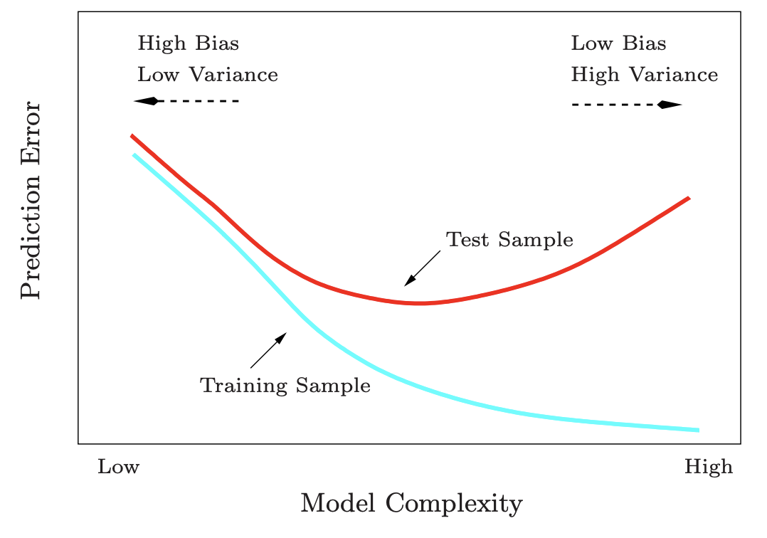
bias-variance-tradeoff — (from *The Elements of Statistical Learning, Section 2*)

In general, the more complex a model, the easier it is to overfit to a training dataset, which results in higher variance and subsequently higher error on a test dataset. In contrast, the more simple a model, the more bias is expected due to limitations of the model itself, and thus also a higher error on a test dataset.

Overfitting and underfitting can also be seen in the context of one model - if you train the model for too long, you may end up overfitting, and if you train for too little, you may end up underfitting. In either case, an engineer must be careful to choose an appropriately complex model and training time for each problem they face - no amount of fancy tricks can solve a non-ideal model choice in the long run.

Wrap-up

In this article, we’ve covered the very basics of supervised learning, starting with simple terms relating to classification and regression, simple models for each of these types of problems, and a small discussion about the bias-variance tradeoff and how it relates to model complexity and selection.

If you’ve made it this far, thank for reading through as always! There is obviously much more to supervised learning than what was covered in this article - I’ll spend some time in the next few articles tackling some more items here. For the next part of this series, I’ll dive deeper into a field we discussed in this article - that of linear classification. Stay tuned!