Advanced Generative AI (Vision Series): ProGAN
Introduction
In my previous article, I covered the Vector Quantized Variational Auto Encoder, or the VQ-VAE. In line with my previous series, this time we’ll cover an advanced generative AI model that falls into the family of Generative Adversarial Networks - otherwise known as GANs.
This article explores an extension to the traditional GAN known as the Progressive GAN or ProGAN. The ProGAN uses a progressive structure in the generator and discriminator that allows for the generation of images with much higher resolution and detail than previous architectures.
ProGAN
The ProGAN follows the GAN by roughly 4 years, and relies heavily on top of the fundamental backbone of the GAN. If you’d like a review of the concepts behind the GAN, you can check out my earlier article here - for this article I’ll only provide a quick review before going through the theory. In those 5 years, a lot of research had been done on GANs but training was still largely unstable and limited by output size.
The ProGAN addresses this issue by working “from the bottom-up”. By starting at lower image resolutions, and then adding details in a progressive manner, the ProGAN is able to achieve much more stable training while also being able to generate higher resolution images with more ease.
Setup
As in the traditional GAN architecture, the ProGAN consists of a generator model
and a discriminator model
. The objective of the GAN is to find a satisfactory equilibrium for the joint value function
For the ProGAN, we will modify the training method by adding in layers to the discriminator and generator throughout training. We’ll add layers in a symmetric manner to both the discriminator and generator, and ensure that the manner in which we add layers doesn’t significantly change the previous trained layers in our model. We’ll also use a modified loss function based off another GAN paper called the Wasserstein loss. Let’s see how we implement all this in practice.
Progressive Growing
We’ll start our network at 4x4 resolution. To implement progressive growing, we’ll train the network at the current resolution for a set number of steps. Then, when we want to add in a new layer (to progress the resolution), we’ll “fade” in the new layer with a parameter . Here, will represent how much of the new layer’s output we will use in the overall output. In mathematical terms, if the lower resolution output was and the higher resolution output that we’re fading in is , we’ll output scaled values , and use similarly interpolated images between the higher resolution and lower resolution for the ground truth. We’ll gradually scale from to , and hopefully in doing so we won’t create too much of a shock in the network with the added layers.
One other consideration is that the batch size of images must also change throughout training. As we process larger and larger images, we require less data for gradient updates, and in fact larger batch sizes may be more prone to instability issues due to the size of the gradient updates. Therefore, it becomes necessary to also maintain a schedule of batch sizes that we’ll use as our network resolution becomes larger.
Since we’re training by resolution, we’ll require a decent number of epochs for each resolution to train to a point of stability (we’ll use 10 for now to make training faster).
Equalized Learning Rate
This section is a slight misnomer - the actual item we’re discussing here is scaling the parameters of the neural network to ensure equal learning rates. In theory, if some parameters in our network have a larger dynamic range (they take on a larger range of values during training), those parameters take longer to learn. The ProGAN paper builds off this idea by first initializing parameters from
, and then scaling the weights dynamically based on He’s initializer, which uses a constant
where
represents the number of input channels and
represents the kernel size for that filter. We’ll use this scaled version of the parameters for every convolutional layer in our model.
PixelNorm
One other scenario the ProGAN authors address is the case where the magnitudes of the values in the generator and discriminator spiral out of control. To prevent this outcome, we’ll normalize the feature vector for each pixel to unit length after each convolutional layer. In mathematical terms,
Here,
,
is the number of channels, and
and
represent pixels over the original features and the normalized features respectively. If you think about this in terms of an example feature of size 512x8x8, we’re essentially normalizing over the channel dimension of size 512, so that the vector associated with each pixel in the 8x8 “image” is normalized.
Minibatch Standard Deviation
The authors also introduce a solution to the variation problem some GANs face - as images become larger, GANs normally tend to suffer in the variety of the generated images as it becomes easier to model a few good outputs instead of many outputs. To combat this, the authors suggest normalizing the discriminator over each minibatch by computing statistics by feature and adding this as extra information for the network.
To implement this, we’ll simply compute the standard deviation for each feature in each spatial location in the minibatch. Then we’ll average these values over all features and locations to arrive at a single constant value, which we’ll replicate and append to the network as a vector for each spatial location and batch example.
Wasserstein Loss
Finally, the authors use a loss function introduced in the WGAN-gp. This loss is based off Wasserstein loss - a theoretical improvement to the original GAN loss that improves the convergence of the generator. The WGAN-gp loss simply adds a small penalty to the Wasserstein loss to encourage better gradients. I won’t go into the derivation for this loss function, but the general form of our new loss is as follows
where the last term effectively constrains the gradients we compute to be unit vectors. In practice,
is usually found to work well.
The authors also introduce a fourth term to this loss, the purpose of which is to keep the discriminator output from drifting away from zero. The new loss with this fourth term added is as follows
where
.
Implementation
Most of the detail in this article will be in the actual code. For the next few sections, we’ll implement each part of the ProGAN step by step, taking care to explain each part in turn.
Equalized Learning Rate
To implement the parameter scaling from earlier, we’ll define a custom WSConv2d layer that’ll inherit from the original Conv2d and implement the scaling operation accordingly.
class WSConv2d(nn.Module):

def __init__(self, in_channels, out_channels, kernel_size=3, stride=1, padding=1):
    super(WSConv2d, self).__init__()
    self.conv = nn.Conv2d(in_channels, out_channels, kernel_size, stride, padding)
    self.scale = (2 / (in_channels * (kernel_size ** 2))) ** 0.5
    self.bias = self.conv.bias
    self.conv.bias = None

    nn.init.normal_(self.conv.weight)
    nn.init.zeros_(self.bias)

def forward(self, x):
    return self.conv(x * self.scale) + self.bias.view(1, self.bias.shape[0], 1, 1)
The scaling constant calculation is straightforward once we have all the necessary variables. We also replace the original Conv2d bias with our own because we only want to apply the scaling operation to the weight vectors, not the bias vectors.
PixelNorm
We also need to implement a custom normalization layer for the PixelNorm idea we discussed earlier. The naive way would be using a for loop, but we can take advantage of PyTorch’s parallelism with tensors to implement this in a nicer fashion.
class PixelNorm(nn.Module):
    def forward(self, x):
        return x/torch.sqrt(torch.mean(x ** 2, dim=1, keepdim=True) + 1e-8)
Here, the dimension associated with dim=1 represents our channels, and PyTorch allows us to compute operations over this dimension quite nicely for any tensor.
Progressive Growing
For both the Generator and Discriminator, we’ll need a ConvBlock, similar to our original implementation from the first article. This ConvBlock will consist of two WSConv2d layers back-to-back, along with a PixelNorm depending upon if the block is in the generator or the discriminator.
class ConvBlock(nn.Module):
    def __init__(self, in_channels, out_channels, use_pixelnorm=True):
        super(ConvBlock, self).__init__()

        self.conv1 = WSConv2d(in_channels, out_channels)
        self.conv2 = WSConv2d(out_channels, out_channels)
        self.pn = PixelNorm() if use_pixelnorm else nn.Identity()

    def forward(self, x):
        x = F.leaky_relu(self.pn(self.conv1(x)), 0.2)
        x = F.leaky_relu(self.pn(self.conv2(x)), 0.2)
        return x
To implement progressive growing, we’ll have the .forward() methods of both the generator and discriminator take inputs related to the stage of progressive growth we are at. We’ll also use a parameter alpha to designate the level of interpolation we’d like for the output.
The Generator and Discriminator are pretty much symmetrical, so I’ve included the code for both below
class Generator(nn.Module):
    def __init__(self, args, dim_mults = [1, 1, 1, 1, 2, 4, 4]):
        super(Generator, self).__init__()
        self.args = args

        hidden_dims = [int(args.dim / mult) for mult in dim_mults]

        self.embed = nn.Sequential(
            WSConvTranspose2d(args.latent, args.dim, 4, 1, 0),
            PixelNorm(),
            nn.LeakyReLU(0.2),
            WSConv2d(args.dim, args.dim, 3, 1, 1),
            nn.LeakyReLU(0.2),
            PixelNorm(),
        )

        self.progressive_blocks = nn.ModuleList([
            *[
                ConvBlock(in_f, out_f) for in_f, out_f in zip(hidden_dims[:-1], hidden_dims[1:])
            ],
        ])

        self.out_blocks = nn.ModuleList([
            *[
                WSConv2d(out_f, args.channel_size, 3, 1, 1) for out_f in hidden_dims
            ],
        ])

    def fade(self, lower, higher, alpha):
        return alpha * higher + (1 - alpha) * lower

    def forward(self, x, p, alpha):
        out = self.embed(x)

        for i in range(p):
            out_lower = out
            out = F.interpolate(out, scale_factor=2, mode="bilinear")
            out = self.progressive_blocks[i](out)

        if p > 0:
            out_lower = self.out_blocks[p-1](out_lower)
            out_lower = F.interpolate(out_lower, scale_factor=2, mode="bilinear")
            out = self.out_blocks[p](out)
            final_out = self.fade(out_lower, out, alpha)
        else:
            final_out = self.out_blocks[p](out)

        return F.tanh(final_out)

class Discriminator(nn.Module):
    def __init__(self, args, dim_mults = [1, 1, 1, 1, 2, 4, 4]):
        super(Discriminator, self).__init__()
        self.args = args

        hidden_dims = [int(args.dim / mult) for mult in reversed(dim_mults)]

        self.progressive_blocks = nn.ModuleList([
            *[
                ConvBlock(in_f, out_f, use_pixelnorm=False) for in_f, out_f in zip(hidden_dims[:-1], hidden_dims[1:])
            ],
        ])

        self.in_blocks = nn.ModuleList([
            *[
                WSConv2d(args.channel_size, in_f, 1, 1, 0) for in_f in hidden_dims
            ],
        ])

        self.downsample = nn.AvgPool2d(kernel_size=2, stride=2)

        self.map = nn.Sequential(
            WSConv2d(args.dim + 1, args.dim, 3, 1, 0),
            nn.LeakyReLU(0.2),
            WSConv2d(args.dim, args.latent, 4),
            nn.LeakyReLU(0.2),
        )

        self.linear = WSConv2d(args.latent, 1)

        self.minibatch_stddev = MiniBatchStdDev()

    def fade(self, lower, higher, alpha):
        return alpha * higher + (1 - alpha) * lower

    def forward(self, x, p, alpha):

        for i in range(p, -1, -1):
            rev_p = len(self.progressive_blocks) - i

            if i == p:
                out = self.in_blocks[rev_p](x)

            if i == 0:
                out = self.minibatch_stddev(out)
                out = self.map(out)
            else:
                out = self.progressive_blocks[rev_p](out)

            if i > 0:
                out = self.downsample(out)

                if i == p and alpha < 1:
                    downsampled = self.in_blocks[rev_p + 1](self.downsample(x))
                    out = self.fade(downsampled, out, alpha)

        out = self.linear(out)
        return out
Minibatch Standard Deviation
We’ll also quickly implement a module to compute the standard deviation over minibatches and add the averaged output as a new channel to the input right before the end of the discriminator. Although the paper itself doesn’t mention the idea of groups, the original implementation does, so that’s what we’ll do.
class MiniBatchStdDev(nn.Module):
    def __init__(self, group_size=4):
        super().__init__()
        self.group_size = group_size

    def forward(self, x):
        B, C, H, W = x.shape
        G = min(self.group_size, B) if B % self.group_size == 0 else 1

        y = x.view(G, -1, C, H, W)

        # compute std dev
        y = y - torch.mean(y, dim=0, keepdim=True)
        y = torch.mean(torch.square(y), dim=0)
        y = torch.sqrt(y + 1e-8)

        # average over all other dimensions
        y = torch.mean(y, dim=[1,2,3], keepdim=True)

        # repeat value for feature map
        y = y.repeat(G, 1, H, W)

        # add to input
        return torch.cat([x,y], dim=1)
And with that, we’re done with the implementation of the networks!
Generating Art
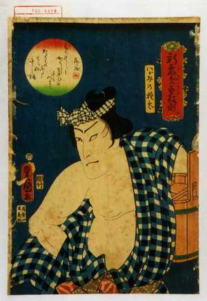
Now that we have every module written, we can put together the training loop and dataset to generate some new artwork. As always, all the experiments below use images from the Japanese Woodblock Print database to better emulate the challenge of handling real datasets in the wild.

Let’s try and generate images like the one above!
As always, I’ll skip the steps of defining the dataset and dataloader since they’re usually pretty simple and instead focus on the training loop for the ProGAN. If you’d like to see that code, you can check out the full repo here .
Let’s define our actual training loop. We’ll iterate through all the resolutions we have, training through n epochs each.
For each batch, we’ll first update the discriminator and then the generator. To compute the discriminator loss, let’s first write a function to compute the gradient penalty from the WGAN-gp loss.
def compute_gradient_penalty(self, d_net, batch, fake, p, alpha):
    B, C, H, W = batch.shape
    beta = torch.rand((B, 1, 1, 1)).repeat(1, C, H, W).to(self.args.device)
    interpolated_images = batch * beta + fake.detach() * (1 - beta)
    interpolated_images.requires_grad_(True)
    preds = d_net(interpolated_images, p, alpha)
    gradient = torch.autograd.grad(
        inputs=interpolated_images,
        outputs=preds,
        grad_outputs=torch.ones_like(preds),
        create_graph=True,
        retain_graph=True,
    )[0]
    gradient = gradient.view(gradient.shape[0], -1)
    norm = gradient.norm(2, dim=1)
    return torch.mean((norm - 1) ** 2)
Then, we can write the discriminator loss and update. The simplified loss function from the Wasserstein loss makes this implementation quite nice.
d_net.zero_grad()

fake_batch = g_net(noise, p, alpha)
dx = d_net(batch, p, alpha).view(-1)
dgz_1 = d_net(fake_batch.detach(), p, alpha).view(-1)
gp = self.compute_gradient_penalty(d_net, batch, fake_batch, p, alpha)
d_loss = torch.mean(dgz_1) - torch.mean(dx)
d_loss += self.args.lambda_gp * gp
d_loss += 0.001 * torch.mean(dx ** 2)

d_loss.backward()
d_optimizer.step()
The generator loss and update are fairly straightforward in comparison
g_net.zero_grad()

fake_batch = g_net(noise, p, alpha)
dgz_2 = d_net(fake_batch, p, alpha).view(-1)
g_loss = -torch.mean(dgz_2)

g_loss.backward()
g_optimizer.step()
Finally, we have to slowly scale
from 0 to 1 throughout training for each resolution. We’ll add some code to do that real quick.
alpha += 2 / (self.args.n * len(self.dataloaders[p]))
alpha = min(alpha, 1)
As per usual, I also included some code to track the outputs of the generator throughout training on the same fixed latent. This time, we’ll have different resolutions of outputs as well. I’ve skipped that code here since it’s the same as always, but it’s available at my public repository if you’d like to take a look.
With that, we’re ready to train! In my experiments, I ran the training for 10 epochs at each resolution, scaling up from a resolution of 4 to 256. The paper suggests using a learning rate of 1e-3 and a batch size of 16 to start, and I use a latent size of 128.
Let’s see how it did! To start, I've created an animation showing how the ProGAN increases resolution and improves over the fixed latent. You can see when the resolution increases because the image quality becomes worse at first. Click the animation again if you'd like to restart it.

Overall, it appears to be doing pretty well at the start! We can see how it starts with the lower level features and then slowly adds onto them. However, we can also see that as we get to higher resolutions the output quality decreases pretty drastically.
Let's see how the final generated outputs look. For each image below, I’ve put a generated image from our ProGAN as well as an image from the dataset that I thought looked similar.

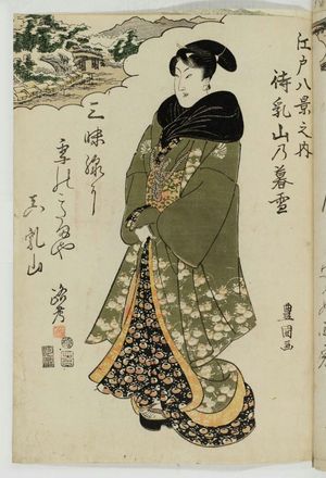
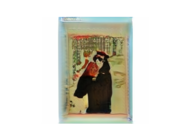
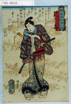

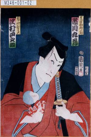


So . . . the images really aren’t that good even compared to the vanilla DCGAN. We can see similarities between some of the dataset images and the generated art above, especially with smaller details like the writing and stamps, but the ProGAN doesn’t seem to be able to make that last step on the higher level features for this dataset. The main reason this is likely happening for this particular dataset is image quality - the larger a network gets it generally becomes more important to have access to quality data.
However, it’s also quite likely that with more training, the outputs of the model would have improved. The ProGAN model takes an incredibly long time to train - I only trained for 60 epochs in total, while the original authors ended up training for almost 10 days in total. If you’re trying this code out on your own, I’d highly recommend trying it out on a more curated dataset with samples that are more similar to each other, or simply allowing more time for the model to converge.
Wrap-up
Although the ProGAN model is relatively simple in concept, there are many implementation details that can be quite complex. Furthermore, as we’ve seen it’s possible that for your dataset the ProGAN is simply not good enough at image generation. In this case, I’d recommend choosing datasets that make the task easier for your GANs, with consistent samples from similar angles / perspectives that are of the same general subject.
If you’ve made it this far, thank for reading through as always! For the next part of this series, I’ll attempt to build on the Progressive GAN and cover a particularly unique and recent improvement on them - the StyleGAN.
If you’d like to check out the full code for this series, you can visit my public repository .